Abstract—A new method for curve machining on 5-axis CNC machine tools is proposed in this paper. It uses the CNC interpolator approach, or called curve interpolator, which can produce accurate tool position as well as tool orientation. The interpolator calculates a new command in real time, the same time period needed for sampling the control-loop feedback devices. It performs two steps in each sampling period: (1) trajectory planning based on a constant feedrate and (2) inverse kinematics transformation based on the structure of the machine. To implement this curve interpolator, a 3-D parametric curve g-code must be defined for 5-axis CNC machining. The comparison for the proposed method and the conventional off-line method in terms of trajectory accuracy feedrate variation are demonstrated in the end of this paper.
Index Terms—CNC, Computer control, Five-axis machining, machine tools
I. INTRODUCTION
T has been known that 5-Axis CNC (Computer Numerical Control) machining for molds and dies produces higher metal removal rates and improved surface finish, compared with conventional 3-axis machining [1-4]. However, the current methods for 5-axis machining utilize off-line part programming approaches by which the CAD system divides the surface into a set of line segments that approximates the surface at the desired tolerance [5-9]. These line segments are further processed by post processors to produce straight-line g-codes which constitute the commands needed to control the machine. In the CNC system, these linear g-codes are fed into the interpolator that makes a linear motion for the curve. Chou and Yang [10] provided a mathematical formulation for an Euler-angle-type 5-axis machine to track a parametric curve. Their work interpolated the curve correctly, but the required tool orientations were assumed to be given from CAD files.
Manuscript received December 28, 2010; revised January 31, 2011. This work was supported in part by National Science Council, Taiwan, R. O. C. under the Grant NSC 98-2221-E-194 -045 -MY2.
Rong-Shine Lin*, Associate Professor in the Department of Mechanical Engineering, National Chung Cheng University, Chia-Yi, Taiwan 62102, R.O.C. (corresponding author e-mail: [email protected], phone: +886-5272-0411 ext. 33300; fax: +886-5272-0589..
Shyh-Leh Chen, Professor in the Department of Mechanical Engineering, National Chung Cheng University, Chia-Yi, Taiwan 62102, R.O.C.
J-H Liao, Graduate student in the Dept. of Mechanical Engineering, National Chung Cheng University, Chia-Yi, Taiwan 62102, R.O.C..
This off-line approach for 5-axis machining either assumes a constant tool orientation along each segment, or assumes a linear change in the tool orientation between successive end-points. The constant orientation algorithm causes severe roughness around the end-points along the surface since the orientation changes are abrupt at these points. The linear orientation algorithm produces a better surface, but still cannot interpolate the orientations accurately between end points. This is because that the changes of the orientation along a curve are not necessarily linear and substantially causes machining errors. An additional drawback of the off-line methods is that the cutter accelerates and decelerates at each segment, which increases the surface non-uniformity and subsequently increases the cutting time [11, 12].
To overcome these drawbacks, this paper proposes an algorithm for real-time 5-axis interpolator that generates both tool orientation and position precisely. This interpolator can produce desired trajectories for 5-axis curve machining. The interpolator calculates new commands for 5-axis controllers in the same time period, which is needed for sampling the control-loop feedback devices. The interpolator performs two steps in each sampling period: (1) trajectory planning based on a constant feedrate, and (2) inverse kinematics transformation based on the structure of the machine.
The input to the interpolator is a new defined g-code (i.e., a CNC instruction), which contains the geometric information of the part surface as well as the cutting conditions, such as the feedrate, the spindle speed, the specific tool, etc. The interpolator begins with trajectory planning portion, which generates the position (x,y,z) and the orientation (Ox,Oy,Oz) of the cutter based on the curve
geometry and the specified constant feedrate in each sampling period. This is a generic, machine independent algorithm. Based on the calculated cutter's position and orientation, the reference values of the five axes can be obtained by the inverse kinematics transformation, an algorithm which depends upon the structure of each particular machine.
To use the proposed interpolator for 5-axis curve machining, new g-codes must be defined for programming the part program. In this paper, the 3-D parametric curve g-code for 5-axis machining will be given and illustrated by examples. The accuracy and feedrate analyses for the interpolating results will be discussed in the end of the paper.
Advanced Curve Machining Method for 5-Axis
CNC Machine Tools
Rong-Shine Lin*, Shyh-Leh Chen, and J-H Liao
II. 5-AXIS CNCSYSTEMS
The motion control kernel of the CNC system consists of a real-time interpolator and a servo-controller that dominates the axis coordination and motion accuracy. Figure 1 shows the structure of the CNC motion control kernel. As shown in the figure, the input to the CNC is the g-code type of part program. The major function of the real-time interpolator is to generate the reference commands for the servo-controller, which coordinates the multi-axis motion simultaneously.
The real-time interpolator for five-axis CNCs consists of the trajectory/ orientation planning module and the inverse kinematics transformation module. The trajectory/orientation planning generates the tool position (x,y,z) and orientation (Ox,Oy,Oz) based on the machining trajectory, or called tool
path. The six (x,y,z,Ox,Oy,Oz) variables have to be
transformed into five (X,Y,Z,A,B), which are the reference inputs for five servo-controllers. This transformation is called inverse kinematics transformation where the solution depends on the structure of a particular machine.
A. Tool Trajectory
In order to produce smooth curves for a feed-drive CNC system, the machining feedrate (V) must be constant when the cutter tracks the desired trajectory. To keep the constant feedrate, the cutting tool has to move a constant distance relative to the workpiece in each sampling period of the interpolator. The desired tool trajectory can be expressed as a parametric curve C (u) and denoted as,
kˆ ) u ( z jˆ ) u ( y iˆ ) u ( x ) u (
C = + + (1)
where ⎪ ⎪ ⎩ ⎪ ⎪ ⎨ ⎧ + + + + = + + + + = + + + + = − − − − − − 0 1 1 n 1 n n n 0 1 1 n 1 n n n 0 1 1 n 1 n n n c u c u c u c ) u ( z b u b u b u b ) u ( y a u a u a u a ) u ( x L L L
Based on the parametric curve, the interpolator calculates the tool position at each sampling period (T). However, the constant change in the parameter u in the parametric domain does not guarantee the constant length in the Cartesian domain, and consequently does not guarantee a constant feedrate. To obtain the constant feedrate, the conversion between the parameter u and the constant distance that the tool moves at each sampling period has to be derived, A solution based on Taylor's expansion is used to obtain the value of u that corresponds to equal trajectory length of the parametric curve. HOT ) t -(t dt u d 2 1 ) t -(t dt du u u 2 i 1 i t t 2 2 i 1 i t t i 1 i i i + + + = + = + =
+ (2)
where HOT is the high order term and usually can be neglected. By substituting into feedrate and sampling time, the above equation becomes,
4 i u u 2 2 2 2 i u u i 1 i du dC(u) 2 du C(u) d du dC(u) T V -du dC(u) T V u u = = + ⎟⎟ ⎠ ⎞ ⎜⎜ ⎝ ⎛ ⋅ ⋅ ⋅ +
= (3)
This equation shows the function of u in terms of a constant length (VT), which is the distance that the tool moves during one sampling period T.
B. Tool Orientation
5-Axis machine tools can control not only the tool position, but the tool orientation. The above tool trajectory planning calculates tool positions. The tool orientation can be obtained by calculating the main normal for the curve. The normal direction is perpendicular to the curve tangent. The unit tangent vector can be determined by,
) ( C ) ( C T u u ′ ′ = v (4) From the differential geometry, the rate change of tangent
along the curve is the curve normal and denoted as, N
dS T dv =κv
(5) where κ is the radius of curvature and Nv is the unit normal
vector. By rearranging the above equation, the unit normal can be obtained,
dS T d with dS T d 1 N v v
v = κ=
κ (6)
This normal vector is the tool orientation for a desired curve and can be used for 5-axis end-milling machining.
C. Inverse Kinematics
The above curve trajectory and normal represents the tool position(x,y,z) and orientation(Ox,Oy,Oz), respectively.
However, the 5-axis machine tool has only 5 axes to be controlled. The transformation from the tool position and orientation into 5-axis reference positions uses inverse kinematics techniques.
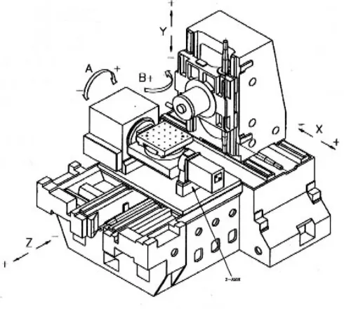
The inverse kinematics transformation depends on the structure of the machine. The machine structure used for our derivations is shown in Fig. 2, which is a horizontal 5-axis machine tool. As shown in Fig. 2, two rotation axes are place on top of the Z-axis table. The tilting axis is rotating along the X axis, and denoted as A axis. The rotation axis is installed on top of the tilting axis and rotating along the Y axis, which denoted as B axis. In this case, the tool axis is fixed on the orientation [0,0,1]. To produce the part surfaces with tool orientation control on this five-axis machine, the part surface normal direction needs to be rotated into the fixed tool orientation [0,0,1].
transformation is to calculate the required rotation angles for tool orientations. We assume that the required tilting and rotating angles for this motion are A and B, respectively. A transformation equation with two rotations can be obtained in terms of the Homogeneous Transformation Matrices, R(x, A) • R(y, B) • T
z y x,O ,O ,1]
[O = [0,0,1,1]T (7) where R(x, A) is the Homogeneous transformation matrix that rotates along the x axis with an angle A, shown in Eq. (8) in detail. Likewise, R(y, B) represents the notation of rotating along Y axis with an angle B. [0,0,1,1]T is the transpose matrix of [0,0,1,1], likewise T
z y x,O ,O ,1]
[O . The
detailed expression for Equation (7) is shown below,
⎥ ⎥ ⎥ ⎥ ⎦ ⎤ ⎢ ⎢ ⎢ ⎢ ⎣ ⎡ = ⎥ ⎥ ⎥ ⎥ ⎦ ⎤ ⎢ ⎢ ⎢ ⎢ ⎣ ⎡ • ⎥ ⎥ ⎥ ⎥ ⎦ ⎤ ⎢ ⎢ ⎢ ⎢ ⎣ ⎡ − • ⎥ ⎥ ⎥ ⎥ ⎦ ⎤ ⎢ ⎢ ⎢ ⎢ ⎣ ⎡ − 1 1 0 0 1 O O O 1 0 0 0 0 B cos 0 B sin 0 0 1 0 0 B sin 0 B cos 1 0 0 0 0 A cos A sin 0 0 A sin A cos 0 0 0 0 1 z y x (8)
Two unknowns, A and B, in Eq. (8) can be solved for
) O O ( tan A z y 1 −
= and )
O O O ( tan B 2 z 2 y x 1 + −
= − (9)
After two simultaneously rotating motions, the tool position has been moved to a new location. Therefore, the next step is to find the distance between this tool location and the desired trajectory location. The determined distance in terms of XYZ coordinate system is the reference position for three translational axes. Using Homogeneous Transformation notation, this distance can be calculated as
[
]
[
]
TT 1 , z , y , x ) Qz , Qy , Qx ( T ) B , y ( R ) Tz , Ty , Tx ( T ) A , x ( R ) OTz , OTy , OTx ( T 1 , Z , Y , X • • • • •
= (10)
where T(a,b,c) represents a linear translation along a vector of [a,b,c] in the XYZ coordinate system. In Eq. (10) (x,y,z) is the tool location on the curve in terms of the part coordinate system. (Qx,Qy,Qz) is a relative distance between
the part coordinate system and the rotating table (B-axis) coordinate system. (Tx,Ty,Tz) is a relative distance between
the rotating coordinate system and the tilting table (A-axis) coordinate system. (OTx,OTy,OTz) is a relative distance
between the tilting coordinate system to the tool coordinate system. Therefore, Equation (10) can be expressed as
⎥ ⎥ ⎥ ⎥ ⎦ ⎤ ⎢ ⎢ ⎢ ⎢ ⎣ ⎡ • ⎥ ⎥ ⎥ ⎥ ⎦ ⎤ ⎢ ⎢ ⎢ ⎢ ⎣ ⎡ • ⎥ ⎥ ⎥ ⎥ ⎦ ⎤ ⎢ ⎢ ⎢ ⎢ ⎣ ⎡ − • ⎥ ⎥ ⎥ ⎥ ⎦ ⎤ ⎢ ⎢ ⎢ ⎢ ⎣ ⎡ • ⎥ ⎥ ⎥ ⎥ ⎦ ⎤ ⎢ ⎢ ⎢ ⎢ ⎣ ⎡ − • ⎥ ⎥ ⎥ ⎥ ⎦ ⎤ ⎢ ⎢ ⎢ ⎢ ⎣ ⎡ = ⎥ ⎥ ⎥ ⎥ ⎦ ⎤ ⎢ ⎢ ⎢ ⎢ ⎣ ⎡ 1 z y x 1 0 0 0 Qz 1 0 0 Qy 0 1 0 Qx 0 0 1 1 0 0 0 0 B cos 0 B sin 0 0 1 0 0 B sin 0 B cos 1 0 0 0 Tz 1 0 0 Ty 0 1 0 Tx 0 0 1 1 0 0 0 0 A cos A sin 0 0 A sin A cos 0 0 0 0 1 1 0 0 0 OTz 1 0 0 OTy 0 1 0 OTx 0 0 1 1 Z Y X (11)
The (X,Y,Z) in Eq. (11) and the (A,B) in Equation (9) are the solutions of inverse kinematics transformation , which are the reference commands for five-axis servo-controllers.
The controllers usually perform a specified control algorithm, e.g., PID control, to reduce the axial tracking errors.
III. MOTION CODE
A. Rational Bezier Curve
Free-form curves or surfaces have been widely used for product design in recent years. One of the convenient models for free-form curve is the parametric form. This rearch uses rational Bezier curve, a parametric curve, for the CNC input format. A rational Bezier curve can be denoted as,
0 w (u) Br w (u) Br p w
C(u) n i
0 i n i i n 0 i n i i i ≥ =
∑
∑
== , (12)
where u is the parameter; p is the control point that controls the shape of the curve. Br is the blending function, which is a Bernstein Polynomial with order n-1. w is a wieght that adjusts the curve’s weighting.
B. G-code Format
In order to descirbe a rational Bezier curve, the motion code, or called g-code, includes the control points and weights. A newly defined g-code format for the curve is shown below,
N01 G701 p1x p1y p1z w1 m p2x p2y p2z w2 p3x p3y p3z w3 p4x p4y p4z w4
G701 is used for the curve interpoator motion word and N is the block number. The control point in the Cartisent Coordinated system is followed by the motion word, as well as the associated wieght. m is the number of control points to be used in this motion code. For this example, m is 4 and therefore, 3 more control points will be needed for this g-code.
An example is demonstrated for the above definition, as shown below.
N01 G701 X0 Y0 Z0 W.8 m4
X50 Y30 Z60 W.5
X80 Y80 Z30 W.2
X130 Y90 Z10 W.7
The result of the curve interpolation for this g-code is shown in Fig. 3.
IV. RESULTS AND DISCUSSIONS
A. Feedrate Analyses
equation (X,Y,Z axes), the axial velocity can be obtained and shown in Fig.4. Likewise, Figure 5 shows the angular velocities for the rotating axes (A and B).
In order to see the tool motion velocity, the distance for each sampling is calculated and shown in the Fig. 6. The velocity is between 0.5988 m/sec and 0.6002 m/sec, which keeps very close to the programmed feedrate 0.6m/sec. The calculation time for the curve interpolator for each iteration is 0.0044, which is less than the system sampling time and satisfies the CNC system regulation.
B. Accuracy Analyses
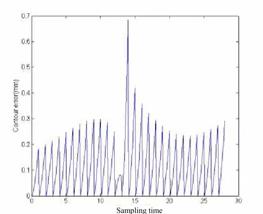
The interpolating accuracy depends on the precision of the tool motion relative to the desired curve. The error between the these two trajectories is defined as the contour error. A scheme of the contour error is shown in the Fig.7. By analyzing the contour errors for the developed curve interpolator, as shown in Fig. 8, the maximum contour error is 0.683mm and the average contour error is 0.118mm.
In contrast, the conventional curve machining uses off-line decomposition that causes large errors. With the same example above, it is decomposed into 21 line segments and subsequently feeds the 21 G01 motion codes into the CNC system. The contour errors for this machining method are shown in Fig. 9. The maximum error is 4.369mm. The error, in this machining method, can be reduced by increasing the number of decomposed line segments; however, it causes the longer machining time, as well as the mismatched tool orientations.
V. CONCLUSIONS
This paper presents a new method for curve machining on 5-axis CNC machine tools, using the CNC interpolator approach. The interpolator calculates in real time a new command in the same time period needed for sampling the control-loop feedback devices. It performs two steps in each sampling period: (1) tool trajectory and orientation planning based on a constant feedrate and (2) inverse kinematics transformation based on the structure of the machine. The interpolating result shows that it can produce high accurate tool positions as well as tool orientations.
To implement this curve interpolator, a 3-D parametric curve g-code must be defined for 5-axis machining. This paper defines the parametric curve in the rational Bezier format. The interpolating calculation time for a curve with 4 control point for each iteration is 0.0044, which is less than the system sampling time and satisfies the CNC system regulation. If a curve with more control points, the computation load will be increased due to the complexity of the higher order polynomials. It is suggested that the curve should be described under 6 control points, which uses the blending function with 5th order polynomial.
ACKNOWLEDGMENT
The authors would like to acknowledge the financial support of the National Science Council, Taiwan, R. O. C. under the grant: NSC 98-2221-E-194 -045 -MY2.
REFERENCES
[1] Gani, E., Jruth, J., Vanherck, P., and Lauwers, B., “A Geometrical Model of the Cut in The Five-Axis Milling Accounting for the Influence of Tool Orientation,” Int. J. of Manuf. Technol, Vol. 13, 1997, pp. 677-684.
[2] Jensen, C. G. and Anderson, D. C., "Accurate Tool Placement and Orientation for Finish Surface Machining", ASME Winter Annual Meeting, 1992, pp. 127-145.
[3] Sprow, Eugene E., "Set Up to Five-Axis Programming", Manufacturing Engineering, November, 1993, pp. 55-60.
[4] Vickers, G. W. and Quan, K. W., "Ball-Mills Versus End-Mills for Curved Surface Machining", ASME Journal of Engineering for Industry, Vol. 111 Feb., 1989, pp. 22-26.
[5] Huang, Y. and Oliver, J., “Integrated Simulation, Error Assessment, and Tool-Path Correction for Five-Axis NC Milling,” J. of Manuf. Systems, Vol. 14, No. 5, 1995, pp. 331-344.
[6] Renker, H., "Collision-Free Five-Axis Milling of Twisted Ruled Surfaces", Annals of the CIRP Vol. 42/1/1993, pp. 457-461.
[7] Sanbandan, K. and Wang, K., "Five-Axis Swept Volumes for Graphic NC Simulation and Verification", ASME the 15th Design Automation Conference, DE Vol. 19-1, 1989, pp. 143-150.
[8] Wang, W. and Wang, K., "Real-Time Verification of Multiaxis NC Programs with Raster Graphics", Proceedings of IEEE International Conference on Robotics and Automation, 1986, pp. 166-171.
[9] You, C. and Chu, C., “Tool-Path Verification in Five-Axis Machining of Sculptured Surfaces,” Int. J. of Manuf. Technol, Vol. 13, 1997, pp. 248-255.
[10]Chou, J. and Yang, D., "On the Generation of Coordinated Motion of Five-Axis CNC/CMM Machines", Journal of Engineering for Industry, Vol. 114, Feb., 1992, pp. 15-22.
[11]Shpitalni, M., Koren, Y., and Lo, C.C., "Real-Time Curve Interpolator", Computer-Aided Design, Vol. 26. No. 11, 1994, pp. 832-838. [12]Lin, R. and Koren, Y., "Real-Time Interpolators for Multi-Axis CNC
Machine Tools", CIRP Journal of Manufacturing Systems, Vol. 25. No. 2, 1996, pp. 145-149.
[13]Liu, X. B., Fahad Ahmad, Kazuo Yamazaki, Masahiko Mori,” Adaptive interpolation scheme for NURBS curves with the integration of machining dynamics”, International Journal of Machine Tools & Manufacture 45 (2005) 433–444, 2005.
Trajectory Orientation Planning
Inverse Kinematics Transformation
Servo Controller G-code Part Program
R
eal
-T
im
e I
nte
rp
olat
or
C
N
C
M
otio
n C
on
tro
l K
er
ne
l
[image:5.595.300.552.56.256.2]5-Axis Machine Tool
[image:5.595.82.239.62.297.2]Figure 1. The proposed interpolator for 5-axis curve machining
[image:5.595.307.543.311.489.2]Figure 2. The structure of the horizontal five-axis machine tool.
Figure 3. The interpolating result of a rational Bezier curve
Figure 4. The velocities for 3 translational axes
Figure 5. The angular velocities for 2 rotating axes
(mm) (mm)
[image:5.595.48.293.355.575.2] [image:5.595.319.537.534.713.2]Figure 6. The tool velocities during CNC motion
[image:6.595.50.286.62.238.2]Figure 7. The contour error between the desired curve and the interpolated trajectory
Figure 8. The contours for the interpolated results
Figure 9. The contours for the conventional G01 method
Sampling time
[image:6.595.50.316.397.613.2]