Dynamic Modeling and Adaptive Control of
a Cable-suspended Robot
Abstract
—
The level adjustment of cable-driven parallel mechanism is challenging due to the difficulty in obtaining an accurate mathematical model and the fact that different sources of uncertainties exist in the adjustment process. This paper presents application of an adaptive control scheme for a cable suspended robot to handle uncertainties in mass and moments of inertia of end effecter. In section II dynamic equations of motion are derived and the constraints are utilized to obtain the complete required equations. In section III inverse dynamic controller and adaptive controller are presented. Simulations results presented in section IV show the effectiveness of the adaptive controller when there is no enough knowledge about system parameters.Index Terms—Cable-Suspended Robots, Inverse dynamic Control, Adaptive Control, Positive Tension
I. INTRODUCTION
n recent years, robots have made tremendous inroads into industries for manufacturing and assembly. However, for long reach robotics such as inspection and repair in shipyards and airplane hangars, application of robotics is still in its infancy. Conventional robots with serial or parallel structures are impractical for these applications since the workspace requirements are higher than what the conventional robots can provide. For these reasons, cable suspended robots have received attention and have been recently studied.
Cable-suspended robots can be considered as special parallel manipulators in which the end-effecter is supported by n cables with n tensioning motors. These robots can be made lighter, stiffer, safer, and more economical than traditional serial ones since their primary structure consists of lightweight and high load-bearing cables. On the other hand, one major disadvantage is that the cables can only exert tension and cannot push the end-effecter. Therefore, modeling, workspace analysis, and design of cable robots are different from parallel manipulators. Fattah and Agrawal [1] presented a workspace analysis methodology that can be applied for optimal design of cable-suspended planar parallel robots. The workspace and global condition index were used as the objective functions to optimize the design parameters. Alp and Agrawal [2] described kinematic and dynamic models, workspace and trajectory planning, for these robots.
Manuscript revised March 06, 2011. This work was supported by Shiraz University of Technology, department of mechanical and aerospace engineering, P. O. BOX (71555-313), Shiraz, Iran.
M. Zarebidoki is with the Shiraz University of Technology, Shiraz, Iran (phone: +98-913-3575403; fax: 0711-7264102; e-mail:[email protected]).
A. Lotfavar is with Shiraz University of Technology, Shiraz, IRAN. (e-mail: [email protected]).
H. R. Fahham is with the Mechanical Engineering Department, University of Shiraz, (e-mail: [email protected])
Control of this kind of robots has attracted the attention many researchers, mostly because of its great impact on the efficiency of the robotic systems. Several control methods have been proposed for parallel manipulators. However, only a few of the proposed topologies can be implemented in cable driven parallel manipulators. Most of the proposed control schemes are based on dynamic model of the robot. Representatives of such inverse dynamic control schemes can be viewed in [3], [4] and [5]. Moreover, Fang et al. [6] have proposed a motion control scheme on cable length coordinates, De Luca et al. [7] have presented a proportional and derivative (PD) controller with on-line gravity compensation for robots with elastic joints, Ryeok and Agrawal [8] developed a method for control based on feedback linearization, Ryeok et al. [9] have designed a two level controller for a helicopter carrying a payload using a cable suspended robot, Zi et al. [10] implemented inverse dynamic control using fuzzy neural network type 2 to these robots, Oh et al. [11] used robust control for two-stage cable robots, Oh and agrawal [12-16] proposed Lyapunov Based PD-like control and Nonlinear Sliding Mode control for cable-based robots, and Duchaine et al. [17] have proposed an approach to the control of manipulators using a computationally efficient-model-based predictive control scheme. This paper presents a different control topology examined for possible implementation on cable-suspended robots using an adaptive control scheme. The proposed controller structure guarantees fully tension forces on the cables, in a more trusted fashion, and is capable to fulfill the stringent positioning requirements for these type of manipulators.
II. DYNAMICS OF CABLE-SUSPENDED ROBOTS
In this study, the model of a cable-suspended robot consists of a moving platform (MP) that is connected by n cables to points in the inertial frame or base platform (BP). These n cables (Figure 1) connect respectively points
B
1...
B
non the BP to pointsA
1...
A
non the MP. The center of mass of the MP, together with the reference point on the moving platform is located at C. An inertial reference frame Fo(X1,X2,X3)is located at O and a moving reference frame Fc(X1,X2,X3)is located on the MP at C. Figure 2 presents the position vectors related to the ith cable.M. Zarebidoki, A. Lotfavar, and H.R Fahham
Figure 1: A spatial cable-suspended robot.
Figure 2: Position vectors related to the ith cable. Starting from the vector
l
i connecting pointA
i to pointi
B
, according to Figure 2, one obtains:i i
i c Ra b
l (1) Where
l
i is the vector along the ith cable,c
is position vector of point C,a
iis position vector of point Ai andb
iis position vector of point Bi .The unit vector alongl
i is:) (
)
( i i T i i
i i i b a R c b a R c b a R c e
(2)
and the rotation matrix is given by:
) ( ) ( ) ( ) ( ) ( ) ( ) ( ) ( ) ( ) ( ) ( ) cos( ) ( ) ( ) ( ) ( ) ( ) ( ) ( ) ( ) ( ) ( ) ( ) ( ) ( ) ( ) ( ) ( ) ( 2 1 2 1 2 1 3 3 2 1 1 3 3 2 1 3 2 1 3 3 2 1 1 3 3 2 1 3 2 C C C S S S C S S C C S S S S C S S C S C C S C S S C C R (3)
Where
iis rotation angle ofF
cabout xi–axis and S, C denotes Sin and Cos respectively. The angular velocity ofc
F
can be represented as: P 3 2 1
(4)Where
is vector of rotation angles and
iis ith component of angular velocity. 2 1 1 2 1 1 2 3 2 1 cos cos sin 0 cos sin cos 0 sin 0 1 , P
(5)
and its angular acceleration is:
P P 3 2 1
(6)Where
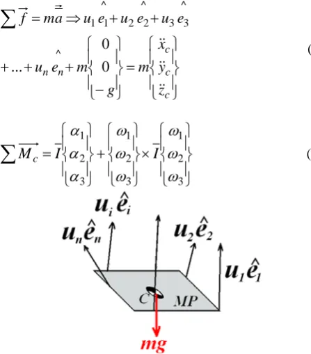
i is ith component of angular acceleration and dot denotes time derivatives. From Newton’s 2nd law (Figure 3):
c c c n n z y x m g m e u e u e u e u a m f 0 0 ... ^ ^ 3 3 ^ 2 2 ^ 1 1 (7)
3 2 1 3 2 1 3 2 1
I IMc (8)
Figure 3: Force vectors on MP
Where m is mass of moving platform (MP).
I
is moment of inertia matrix of moving platform (MP) andgis gravitational acceleration. The equations of motion can be written in a matrix form as:q C G M q M
K
(9) Where ^ 6 6 ^ 5 5 ^ 4 4 ^ 3 3 ^ 2 2 ^ 1 1 ^ 6 ^ 5 ^ 4 ^ 3 ^ 2 ^ 1 ` e a R e a R e a R e a R e a R e a R e e e e e e K (10) } {u1 u2 u3 u4 u5 u6
(11) [image:2.595.308.532.247.502.2]T c
c c y z
x
q{
1
2
3}
(13)
T
g
G{0 0 0 0 0}
(14)
P I P P I q C
0 0 0
(15)
The solution of equation (9) depends on the number of cables. For six cables (non-redundant case), there are six equations and six unknowns. If the six equations are linearly independent, there will be one solution for the problem. For more than six cables (redundant case), system of equations (9) is an underdetermined and has many solutions if KKTis invertible.
In this work, non-redundant cable robots are studied [21]. III. APPLYING CONTROLS ON THE SYSTEM
A. Inverse Dynamic Control
In the control of robots, the inverse dynamic control is one of the control methods employed in non-linear systems with optimized non-sympathetic stability. With regard to the inverse dynamic control law, which is defined in Eqs. (16) and (17) for the robot and Eq. (18) for the controller, U0 is replaced in the first line of Eq. (18) and Eq. (19) has resulted, which can be compared with Eq.(16) and the general law for this control is extracted according to Eq. (20) [17, 18, 20].
) (
1 M q MG Cq
K
U
(16)
)
( 0
1 MU MG Cq
K
U
(17) )
( ) (
0 q K q q K q q
U d D d P d (18)
] ))
( ) ( ( [(
1 M q k q q k q q MG Cq
K
U d d d p d
(19) 0
~ ~
~K qK q
q
M P D (20) With regard to the difference in the function of
3 2 1, ,
, the rate changes related to each iis inevitable;
therefore, KPand KDmatrices in this research, with regard to the robot specifications and constants, are considered the diametric matrices with different rates on diameters. The application of such controller requires inertia matrix, coriolis and centrifugal vectors, gravity acceleration, and system damping calculations [18-20]. These quantities require online calculation because, in this position, the control is based on non-linear response in the present condition of the system; therefore, the mentioned calculations of the quantities are not possible before performing operations and in an offline manner. The inverse dynamic control laws also require that the system dynamic model parameters be recognized precisely and movement complete equations be calculated in real time. The intended model is usually recognized on the bases of
incomplete knowledge present in relation with mechanical parameters and un-modeled dynamics along with a degree of indefiniteness. Also, the unknown rate of dependence of the model to the rate of end effecter load and its load-carrying capacity causes not being able to define an appropriate compensation rate in the controller for it. As a result, the use of other controllers which lack such a limitation is taken into consideration. Even though this control method is able to provide an appropriate function, but compared to the moment disturbances and environmental indefinites, it enjoys high sensitivity. As a result, an adaptive controller can be employed. Adaptive control is used to compensate for parametric uncertainties, suppress constraint uncertainties, and bounded disturbances. This controller, in addition to providing logical responses, enjoys reliability, strength, and appropriate stability in the presence of moment disturbances and uncertainties [22].
B. Adaptive Controller Design
From the robot properties, it can be shown that the dynamic equation, (9) is linear in dynamic parameters.
Y
q
C
G
M
q
M
(21)Where
Y
is a known(
n
r
)
matrix that n is the number of the cables and r is the number of system parameters that there is no enough knowledge about them. Then
is a(
r
1
)
matrix and is equal to:T yz xz xy zz yy
xx
I
I
I
I
I
I
m
]
[
(22)Controllers that can handle regulation tracking problems without the need of knowledge of process parameters are bye themselves an appealing procedure. Such controller schemes belong to the class of adaptive control.
The controller input can be determined by:
MG q C q K q K q M
K
ˆ(d D~ P~) ˆ (23) We assume here thatMˆ,Cˆ and Gˆ have the same functional form asM,C and G with estimated parameters .with respect to equation (21) we can write the following equation.
Y(q,q,q)ˆK (24) Substituting equation (23) into the dynamics of the system gives the following closed-loop error equation.
~ ) , , ( ) ~ ~ ~ (ˆ q K q K q Y q q q
M D P (25) Where(.~)(.)(.)desired
G M M q C C q M M
The error equation in (25) can be rewritten as ~ ( , , ,ˆ)~ )
, , ( ˆ ~ ~
~ 1
q q q q
q q Y M q K q K
q D P (27) This equation can be cast in state space form by choosing
~
., . , ) (
, ~ , ~
2 1 1
1
B A
e i q
q T T T
(28)
With
I B K K
I A
D P
0 , 0
(29)
With choosing the lyapunov function candidate
~ ~ T T
P
V , we can show that if the parameter estimate is updated as
ˆ1TBTP (30)Then the state
of system asymptotically tends to zero. The
is a symmetric positive definite matrix andP
is the solution to the equationATPPAQ, for a given symmetric positive definite matrix Q[23].IV. ANALYSING RESULTS OF THE TREND OF THE TWO CONTROLLERS
After simulation of the two inverse dynamic and adaptive control methods by MATLAB software on the basis of the data obtained from the dynamic analysis of the robot, the results of this section were studied and compared.
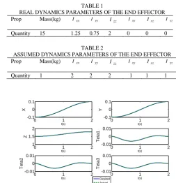
Where there is no uncertainty, the results of the adaptive controller are partly similar to inverse dynamic approach and the error is quickly biased to zero in following a desired path, according to Fig. 4. When there are uncertainty conditions, the results obtained from comparison of adaptive with inverse dynamic are different as depicted in Fig. 5-8. The most important cases considered here as the uncertainties are the probable changes in mass and moment of inertia of the end effecter. Real dynamic parameters of the considered cable- suspended robot are given in table 1. Assumed dynamic parameters to investigate efficiency of adaptive controller are given in table 2. Fig. 9 shows positive tensions in cables by using adaptive controller. Updating of uncertainties in adaptive controller is shown in fig. 10.
V. CONCLUSION
[image:4.595.291.545.74.337.2]In this study the performance of an adaptive controller for a cable-based robot was investigated. The proposed controller is entirely independent on the physical specifications of the robot. Also, the stability of the proposed controller was verified. Simulation results have shown effectiveness of this controller. One of the most interesting things of this controller is that it is independent of the robot specifications in a wide range of variations as well as mass and moment of inertia.
TABLE 1
REAL DYNAMICS PARAMETERS OF THE END EFFECTOR
Prop Mass(kg) Ixx Iyy Izz Ixy Ixz Iyz
Quantity 15 1.25 0.75 2 0 0 0
TABLE 2
ASSUMED DYNAMICS PARAMETERS OF THE END EFFECTOR
Prop Mass(kg) Ixx Iyy Izz Ixy Ixz Iyz
Quantity 1 2 2 2 1 1 1
0 1 2 -0.1
0 0.1
X
t(s)
0 1 2 -0.1
0 0.1
Y
t(s)
0 1 2 1
1.5 2
Z
t(s) 0 1 2
-0.01 0 0.01
Te
ta
1
t(s)
0 1 2 -0.01
0 0.01
Te
ta
2
t(s) 0 1 2
-0.01 0 0.01
Te
ta
3
t(s) Desired
[image:4.595.318.539.383.504.2]Actual
Fig. 4 Following the path without uncertainties via inverse dynamic and adaptive control
0 1 2 -0.2
0 0.2
X
t(s) 0 1 2
-0.2 0 0.2
Y
t(s)
0 1 2 0
2 4
Z
t(s) 0 1 2
-0.01 0 0.01
Te
ta
1
t(s)
0 1 2 -0.01
0 0.01
Te
ta
2
t(s) 0 1 2
-0.01 0 0.01
Te
ta
3
t(s) Desired
[image:4.595.319.537.541.655.2]Actual
Fig. 5 Trajectory tracking by considering uncertainties (variation in mass and moments of inertia) via inverse dynamic control.
0 1 2 -0.1
0 0.1
X
t(s) 0 1 2
-0.1 0 0.1
Y
t(s)
0 1 2 0
2 4
Z
t(s)
0 1 2 -0.01
0 0.01
Te
ta
1
t(s)
0 1 2 -0.01
0 0.01
Teta2
t(s) 0 1 2
-0.01 0 0.01
Te
ta
3
t(s)
0 1 2 -0.2
0 0.2
X
t(s) 0 1 2
-0.2 0 0.2
Y
t(s)
0 1 2 1.6
1.8 2
Z
t(s) 0 1 2
-0.01 0 0.01
Te
ta
1
t(s)
0 1 2 -0.01
0 0.01
Te
ta
2
t(s) 0 1 2
-0.01 0 0.01
Te
ta
3
t(s) Desired
[image:5.595.67.287.49.171.2]Actual
Fig. 7 Trajectory tracking by considering uncertainties (variation in mass and moments of inertia) via adaptive control.
0 1 2 -5
0 5x 10
-5
X
t(s) 0 1 2
-5 0 5x 10
-5
Y
t(s)
0 1 2 0
1 2x 10
-3
Z
t(s) 0 1 2
-5 0 5x 10
-4
Tet
a
1
t(s)
0 1 2 -5
0 5x 10
-4
Te
ta
2
t(s) 0 1 2
-5 0 5x 10
-4
Te
ta
3
[image:5.595.70.287.217.332.2]t(s)
Fig. 8 Error in trajectory tracking by considering uncertainties via adaptive control.
0 1 2
0 50 100
c
abl
e 1
t(s)
0 1 2
0 50 100
c
abl
e 2
t(s)
0 1 2
0 50 100
c
abl
e 3
t(s)
0 1 2
0 50 100
c
abl
e 4
t(s)
0 1 2
0 50 100
c
abl
e 5
t(s)
0 1 2
0 50 100
c
abl
e 6
t(s)
Fig. 9 Tension in cables in the case of using adaptive controller
0 1 2 0
20 40
m
t(s)
0 1 2 2
2.2 2.4
IX
X
t(s)
0 1 2 2
2.2 2.4
IY
Y
t(s) 0 1 2
2 2.2 2.4
IZZ
t(s)
0 0.5 1 1.5 2 0.7
0.8 0.9
IX
Y
t(s)
0 1 2 0
0.51
IX
Z
t(s)
0 1 2 0.6
0.81
IY
Z
t(s)
Fig. 10 Updating uncertainties in adaptive control.
REFERENCES
[1] A. B. Alp, and S. K. Agrawal, Cable Suspended Robots: Design, Planning and Control, Proceedings of International Conference on Robotics and Automation, 2002, Washington, DC, pp. 4275-4280. [2] S. R. Oh, and S. K. Agrawal, A Reference Governor Based
Controller for a Cable Robot under Input Constraints, IEEE Transactions on Control System Technology, Vol. 13, No. 4, pp. 639-645, July, 2005.
[3] P. Gholami, M. Aref, and H. Taghirad, “On the control of the KNTU CDRPM: A cable driven redundant parallel manipulator,” in IEEE/RSJ Int. Conf. IROS, 2008.
[4] A. Trevisani, P. Gallina, and R. L. Williams, “Cable-direct-driven robot (cddr) with passive scara support: Theory and simulation,” J Intell Robot Syst, pp. 73–94, July 2006.
[5] L. Zollo, B. Siciliano, C. Laschi, G. Teti, and P. Dario, “Compliant control for a cable-actuated anthropomorphic robot arm: an experimental validation of different solutions,” in Int. Conf. IROS, May 2002.
[6] S. Fang, D. Franitza, M. Torlo, F. Bekes, and M. Hiller, “Motion control of a tendon-based parallel manipulators using optimal tension distribution”, IEEE/ASME Transactions on Mechatronics, vol. 9, September 2004.
[7] A. D. Luca, B. Siciliano, and L. Zollo, “PD control with on-line gravity compensation for robots with elastic joints: Theory and experiments,” automatica, pp. 1809–1819, May 2005.
[8] S. -R. Oh and S. Agrawal, “Cable suspended planar robots with redundant
cables: Controllers with positive tensions,” IEEE/Transactions and Robotics, vol. 21, January 2005.
[9] S. -R. Oh, J. -C. Ryu, and A. K. Agrawal, “Dynamics and control of a helicopter carrying a payload using a cable-suspended robot” Journal of Mechatronics Design, vol. 128, pp. 1113–1121, September 2006.
[10] B. Zi, B.Y. Duan, J.L. Du, H. Bao, Dynamic modeling and active control of a cable-suspended parallel robot.
[11] LI Cheng-Dong, YI Jian-Qiang, YU Yi, ZHAO Dong-Bin, Inverse Control of Cable-driven Parallel Mechanism Using Type-2 Fuzzy Neural Network.
[12] So-Ryeok Oh and Sunil K. Agrawal. A Control Lyapunov Based PD-like Control of Cable-Suspended Robots
[13] So-Ryeok Oh, Sunil K. Agrawal, Computationally Efficient Feasible Set Points Generation and Control of a Cable Robot. [14] So-Ryeok Oh, Sunil K. Agrawal. Controller design for a
nonredundant cable robot under input constraint
[15] So-Ryeok Oh and Sunil K. Agrawal, Generation of Feasible Set Points and Control of a Cable Robot.
[16] So-Ryeok Oh and Sunil Kumar Agrawal. Nonlinear Sliding Mode Control and Feasible Workspace Analysis for a Cable Suspended Robot with Input Constraints.
[17] V. Duchine, S. Bouchard, and C. M. Gosselin, “Computationally efficient predictive robot control,” IEEE/ASME Transactions On Mechatronics, vol. 12, pp. 570–578, October 2007.
[18] Li Z, Ge SS, Ming A (2007), Adaptive robust motion/force
control of holonomic-constrained nonholonomic mobile
manipulators. IEEE Trans Syst Man Cybern B Cybern 37:607–617.
[19] Li Z, Ge SS, Adams M, Wijesoma WS (2008) Robust adaptive
control of uncertain force/motion constrained nonholonomic mobile manipulators. Automatica 44:776–784. doi: 10.1016/j. automatica.2007.07 012.
[20] Li Z, Ge SS, Wang Z (2008), Robust adaptive control of
coordinated multiple mobile manipulators. Mechatron 18:239–250. doi:10.1016/j.mechatronics.2008.01.001.
[21] Fahham, Hamid Reza, Farid, Mehrdad, Time optimal control of
spatial cable suspended robots considering tension constraints.
[22]Safavi, S. M, Hoshyarmanesh, H, R, Mirian, S, S, Khandan, R,
Design of an adaptive-robust controller for a powder coating robot and its comparison with inverse dynamic approach, Int J Adv Manuf Technol (2009) 45: 1179–1186.
[image:5.595.67.293.376.490.2] [image:5.595.67.286.538.651.2]