Is it better to be mixed in group lending?

Munich Personal RePEc Archive

Is it better to be mixed in group lending?

Reito, Francesco

University of Catania

17 February 2016

Online at

https://mpra.ub.uni-muenchen.de/76129/

1

Is it better to be mixed in group lending?

Francesco Reito

This paper shows that, in a group-lending environment characterized by positive assortative matching, a microfinance institution can achieve a Pareto improvement by promoting negative matching among borrowers. Some new implications are: i) borrowers may be better off under mixed groups; ii) a heterogeneous group lending equilibrium is possible even when individual or homogeneous group equilibria do not exist.

Keywords: group lending, assortative matching, Pareto improvement, outreach

JEL classification numbers: D81, O12

1 Introduction

Group lending is probably the most popular instrument used by microfinance institutions to enforce the repayment of loans. The typical feature of such lending scheme is that borrowers are required to form groups where all members are considered jointly liable for each other’s loan repayment. This mechanism has drawn the attention of a growing literature on credit market imperfections, which shows that group lending can help mitigating the problems of information asymmetry between lenders and borrowers1_{. In particular, the present paper is}

based on the results of Van Tassel (1999) and Ghatak (1999), who argue that group lending always leads to positive assortative matching among micro-entrepreneurs. Namely, in a population of potential borrowers with different risk

* Correspondence: University of Catania, Department of Economics and Business, Corso Italia 55, 95100 Catania, Italy. [email protected].

2 profiles, individuals will sort themselves into homogeneous risk groups. Low-risk individuals would never agree to match with high-risk types, even if side payments among group members are possible.

This paper is built on the adverse selection framework of Ghatak (2000), in which the credit market can be characterized by either underinvestment (Stiglitz and Weiss, 1981), or overinvestment (de Meza and Webb, 1987). Ghatak (2000) considers two types of potential borrowers (safe and risky) and compares their expected utilities under homogeneous or heterogeneous (mixed) matching. In this comparison, both homogeneous and mixed group payoffs are based on the same

financial contract offered by a benevolent microfinance institution (MFI). That is, the contractual terms (individual and joint liability payments) are considered exogenous, irrespective of the final composition of borrowers’ types within the group financed. Under these conditions, the match-payoff function is always supermodular (see Becker, 1973 and Topkis, 1998), and the assortative matching can never be negative. The present paper argues that the payoff of mixed groups should actually be based on a different financial contract. Specifically, the MFI should offer a menu of two different generic contracts, one designed for homogeneous groups, and one for mixed groups. In each of these contracts, the MFI must break even, and so let borrowers choose the type of partner that maximizes their expected payoff. The two main results of the article are:

i) Borrowers may be better off under mixed groups.

This means that a MFI can achieve a Pareto improvement, over the equilibrium characterized by positive assortative matching, by promoting negative matching among borrowers. This conclusion is similar to those derived in some other papers, in particular Sadoulet (1999), Roy Chowdhury (2007) and Guttman (2008), in which the assortative matching may become negative if group lending contracts incorporate the threat of not being refinanced in the future.

3 matching is positive when the number of risky types is low. The reason is that, in an asymmetric information environment, when the homogeneous contract is pooling with a low proportion of risky types, safe borrowers receive a payoff close to their first-best level and, thus, they would never find it profitable to choose a mixed group. If, instead, the number of risky types is large, safe borrowers obtain a payoff close to their reservation level and, if monetary transfers among group members are possible, they may end up being better off under mixed matching.

The paper also shows that, when the potential homogeneous contract is separating

(i.e. groups receive different incentive-compatible contracts), borrowers are indifferent between positive and negative assortative matching. Indeed, in a separating homogeneous equilibrium, safe and risky types obtain their respective full-information profits. And, since in this case the sum of expected returns of homogenous groups (safe-safe and risky-risky) is equal to that of mixed groups (safe-risky and risky-safe), borrowers can achieve the same separating full-information profits in a mixed equilibrium, after ex-post transfers.

The intuition for risk heterogeneity is that, in some circumstances, safe types may be willing to trade some of their low-risk profile in exchange for side payments from risky partners. Mixed matching can be explained by the desire for an intra-group insurance system in addition to joint liability2_{. This kind of insurance may}

operate through transfers of money, food, labour services and gifts among group members. It is well known that credit groups can also serve the role of mutual assistance in rural and poor environments, and empirical evidence of this self-help behaviour is reported by Carpenter and Sadoulet (2000), Dupas and Robinson (2009) and Fafchamps and La Ferrara (2012), either within or outside a formal mutual-credit institution. Besides, though the prevalent view is that group lending leads to homogeneous risk matching (for example Ahlin, 2009), a number of authors report that heterogeneity is in some cases the optimal form of risk-sharing arrangement. For example, evidence on negative matching (or at least the absence

2 _{The model developed in this paper is static and based on universal risk neutrality, thus the}

4 of positive matching) can be found in Van Tassel (2000) himself, Carpenter and Sadoulet (2000), Lensik and Mehrteab (2003), Fafchamps and Gubert (2007), and Berhan et al. (2009) 3_.

The most direct policy implication of the paper is that MFIs, in designing their financial contracts, should also consider the possibility of heterogeneous risk matching as a possible additional self-insurance mechanism.

ii) A mixed equilibrium is possible when homogeneous equilibria do not exist, and even when the reservation income of borrowers is equal to zero.

In the underinvestment setup of Ghatak (2000), safe types cannot receive individual liability contracts because their expected payoff is not sufficient to cover the average loan repayment. This is the classic adverse selection problem, whereby risky projects drive safe types out of the credit market. Ghatak (2000) shows that, if the safe type’s expected return is large enough to guarantee the presence of a joint liability equilibrium, group lending can solve the rationing problem.

On the other hand, underinvestment may obtain even under joint liability in two possible circumstances: a) if the safe type’s expected output does not satisfy the participation constraint in group lending (i.e. the quality of projects is too low); b) if the reservation income of borrowers is zero (a reasonable assumption in underdeveloped contexts). This paper argues that, in such cases, a mixed equilibrium may exist and avoid the credit rationing solution. This implies that mixed lending can also be seen as an instrument for MFIs to promote entrepreneurial activity and alleviate (at least short-term) poverty. This result can be related to the strand of the literature that explores the so-called depth of

3 _{Another possible explanation is offered in the empirical work by Berhabe et al. (2009). In their}

5 outreach, that is the extent to which MFIs are able to reach the poorest segment of the population4_.

It is important to stress that the mixed equilibrium described in the model may be, in some cases, subject to re-matching of borrowers. In fact, since the MFI cannot observe the final composition of groups, if a mixed contract is offered, mixed group members may have the incentive to re-match in homogeneous pairs and choose the mixed contract in order to raise their overall payoffs. This paper shows that the negative assortative matching can be a stable equilibrium if the MFI introduces the threat of withdrawing the mixed contract if loan applications are not compatible with heterogeneous lending.

The theoretical results of the present paper are not only relevant for the microcredit literature, but can also be extended to other contexts that involve the formation of peer groups through a self-selection mechanism. A feature of the model is that, since mixed lending is based on different contractual terms with respect to homogeneous lending, the group payoff function is not always supermodular. As in the marriage market of Becker (1973), the payoff of mixed groups can be large enough to reverse the sign of matching among individuals. In other words, the proportion of low-risk types in the population (the quality of the environment in group lending) can alter the trade-off between substitutability and complementarity in the payoff function. Thus, even though low-risk borrowers are generally considered complements in group lending, they may become substitutes if their proportion is so low as to make homogeneous contracts particularly unfavorable. This conclusion is similar to that obtained in the labor-market equilibrium of Kremer and Maskin (1996), where the matching between firms and employees depends on the distribution of skill types and, in particular, on the relative scarcity of high-skilled workers.

The paper is as follows. Section 2 briefly reviews the underinvestment setup of Ghatak (2000), where projects are classified in terms of second-order stochastic

4 _{A part of the literature on microfinance is concerned with the possibility that the very poor can be}

6 dominance. Section 3 introduces the mixed lending contract. Section 4 derives the sign, positive or negative, of the assortative matching. Section 5 discusses the stability of the mixed equilibrium. Section 6 shows that a mixed equilibrium may exist even when homogeneous equilibria are not possible. Section 7 concludes. The Appendix contains an extension of the overinvestment setup of Ghatak (2000), in which projects are ranked in a first-order stochastic dominance sense.

2 Homogeneous Matching

Ghatak (2000) analyzes a model with two types of risk-neutral potential borrowers, safe and risky, endowed with two different projects. Each project requires a fixed investment of 1. Safe types produce y_s with probabilityp_s, while risky types produce yr ys with probability pr; both projects yield nothing with

the complementary probabilities. Borrowers have no endowment, and thus need a financial loan. As in Stiglitz and Weiss (1981), it is p_s  p_r and

y y p y

ps s  r r  .

There is a risk-neutral benevolent MFI/bank with an opportunity cost of capital of

. Borrowers know each other’s quality, whereas the MFI only knows the exogenous proportion of risky types, (0,1 ) and safe types, 1. This asymmetry of information leads to a typical adverse selection problem. The bank can offer either individual liability or joint liability contracts. The individual contract is a standard debt contract with a fixed repayment, r. In a joint liability contract, instead, borrowers form groups of two members. In this case, a successful borrower, in addition to the individual repayment, r, pays also a joint liability component, c, if the other group member is unsuccessful.

Gathak (2000) assumes that

,

u

y and (A1)

,

u p p

7 where p (1)ps pr, and u is the reservation income of borrowers.

Under (A1), both projects are socially efficient, i.e. their expected output is larger than the resources employed. For (A2), safe types are credit rationed under individual liability lending, i.e. their expected profit is not enough to cover the average loan repayment. Therefore, to avoid the rationing problem, the MFI is forced to offer joint liability contracts.

Under the joint liability contract, (r,c), the expected payoff of a borrower of type

i, by teaming up with a partner of type j, is

c p p r y p c r y p p r y p p c r

Uij( , ) i j( i  ) i(1 j)( i   ) i( i  ) i(1 j) .

Ghatak (2000) shows that, even if side payments among group members are possible5_{, borrowers always choose homogeneous groups, i.e. the assortative}

matching is positive. The reason is as follows. Given the expected loss of safe types from matching with risky partners,

c p p p c r U c r

U_ss( , ) _sr( , ) _s( _s  _r) ,

and the expected gain of risky from matching with safe,

c p p p c r U c r

Urs( , ) rr( , ) r( s  r) ,

it is 0 ) )( ( )] , ( ) , ( [ )] , ( ) , (

[U_ss r c U_sr r c  U_rs r c U_rr r c  p_s p_r p_s  p_r c . (1)

8 That is, the expected loss of safe borrowers is larger than the expected gain of risky borrowers. As a result, safe types would never accept to form a mixed group even after a monetary transfer from risky types.

The MFI maximizes a weighted sum of the expected payoffs of the representative borrowers, i.e.

)

(P : max( 1 ) ( , ) ( , )

,c Uss r c Urr r c r   ,

where  is the relative social weight attached to risky types (which can be different from ).

The joint liability contract must satisfy the borrowers’ limited liability constraint. i.e., a successful borrower must be able to pay both individual and joint liability, or

c r

ys   , (LLC)

where we only need to consider the (lower) return of safe types.

The equilibrium can be separating or pooling. In a separating equilibrium, borrowers receive two different incentive compatibility contracts, (rs,cs) and

) ,

(r_r c_r , which satisfy the following incentive constraints,

) , ( ) ,

( _{s s ss r r}

ss r c U r c

U  , and (ICss)

) , ( ) ,

( _{r r rr s s}

rr r c U r c

U  . (ICrr)

The participation constraints under group lending are

u c r

Uss( , ) , and (PCss)

u c r

9 Separating contracts derive from the bank’s zero-profit conditions on safe and risky groups,

0 )

1

(   

 _{s s s} 

s

sr p p c

p , and (0πCss)

0 )

1

(   

 _{r r r} 

r

rr p p c

p . (0πCrr)

From (0πCss) and (0πCrr), we have rˆ(ps pr 1)/(pspr) and cˆ/(pspr).

Therefore, separating equilibria exist if the (LLC) holds, or ys rˆcˆ, i.e. under

the assumption

   

 

 

r s

p p

y  1 . (A3)

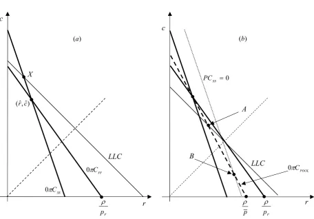
To rule out negative repayments, Ghatak (2000) also assumes that p_s  p_r 1. Figure 1a provides an example in which, under (A3), the (LLC) is above the contract (r,ˆcˆ). The range of separating equilibria is between point X and (r,ˆcˆ) for safe types, and between (r,ˆcˆ) and (/pr,0) for risky types6.

In a pooling equilibrium, borrowers choose the same contract, (r,c), which derives from the bank’s zero-profit condition on the average group,

0 ]

) 1 ( [

] ) 1 ( )[

1

(  psr ps  ps c  prr pr pr c   . (0CPOOL)

Pooling equilibria may exist under a less restrictive assumption on the (LLC), i.e.

u p

p

y( _s/ ) , (A4)

where _[(1_ )_p2 _{ p}2]/_{p p}(01,)

s r s 



 . An example is reported in figure 1b,

where (A3) does not hold, but (A4) holds. In this case, the (LLC) is below (r,ˆcˆ),

10 but above the point where the safe type’s participation constraint becomes binding, i.e. above the intersection between (PC_ss 0) and the bank’s pooling contract line, (0πCPOOL), such as point B. The range of pooling equilibria is the segment between point A and B.

Remark 1: in Ghatak (2000) there is an ex-post incentive compatibility problem, since in the separating contract, (r,ˆcˆ), the amount of joint liability, cˆ, exceeds the individual liability, rˆ. Thus, if (r,ˆcˆ) is offered, there may be the incentive for the group, when one member fails, to announce that both had success and pay 2rˆ

instead of rˆcˆ (this is also true for all pooling equilibria above the 45-degree Figure 1 – Underinvestment (homogeneous equilibria).

a) Separating contracts. b) Pooling contracts. c

(a)

r

) ˆ ,ˆ (r c

LLC

c

r

p



B

(b)

LLC

s

S

C



0

rr

C



0 0CPOOL

A

0



ss

PC

r

p



r

p



11 line in fig. 1a and 1b). A possible theoretical solution, as proposed by Gangopadhyay et al. (2005), may be to impose the additional constraint rc to make incentive compatible to reveal default (i.e. focus on contracts on or below the 45-degree line).

Instead, in the present paper it will be shown that in the mixed matching equilibrium described in the following section, it is always rc, so the full-information outcome can be achieved without imposing the condition that rc.

3 Mixed Matching

A distinctive feature of the model of Section 2 is that the expected utilities of mixed groups, Usr(r,c) and Urs(r,c), derive from the same contract, (r,c),

designed for homogeneous lending. Consequently, in the MFI’s zero-profit conditions, (0Css), (0Crr) and (0CPOOL), the probability of receiving the joint

liability payment, c, is always based on the homogeneous product p_i(1 p_i), for

r s

i , . In contrast, this section argues that the MFI should design two different joint liability contracts, one for homogeneous groups and one specifically for mixed groups. Then, borrowers will choose their most profitable contract and, consequently, will determine the nature of group matching.

The benevolent MFI chooses the mixed contract terms in order to maximize the expected payoffs of potential heterogeneous groups. Since we cannot attach a social weight to a specific mixed group type, the MFI’s program can be written as

)

(P_MIX : max ( , ) ( , )

,c Usr r c Urs r c r  .

The mixed equilibrium contract derives from the MFI’s mixed zero-profit conditions,

0 )

1

(   

 p p c 

r

ps r s , and (0Csr)

0 )

1

(   

 p p c 

r

12 In (0πCsr) and (0πCrs), the bank takes into account the fact that, whenever

borrowers choose a mixed group, the joint liability component, c, is paid with the mixed probability p_i(1p_j).

Solving (0πCsr) and (0πCrs), we obtain

r s r s MIX

MIX c _{p p p p}

r

  

  .

Note that, under mixed lending, the equilibrium contract is pooling and unique, so we have neither separating nor other pooling equilibria in addition to (rMIX,cMIX). As discussed in remark 1, rMIX cMIX, so under mixed matching we do not derive

the ex-post incentive problem of Ghatak (2000).

The equilibrium must satisfy the borrowers’ participation constraints7_{, and the}

mixed limited liability constraint,

r s r s MIX MIX

s r c _{p p p p}

y

   

 2 . (LLCMIX)

The mixed match-output utilities can be written as

               r s r s r s s MIX r s MIX s s MIX MIX

sr r c p y r p p c p y _{p p} p _{p p}

U ( , ) ( ) (1 ) (2 ) , (2a)

               r s r s s r r MIX s r MIX r r MIX MIX

rs r c p y r p p c p y _{p p} p _{p p}

U ( , ) ( ) (1 ) (2 ) . (2b)

The payoffs in (2a) and (2b) are always positive under (LLCMIX).

7 _{It is not necessary to specify the heterogeneous participation constraints because they will be}

13 Remark 2: the model of Section 2 is built on the assumption of universal risk neutrality. Ghatak (2000) shows that risk aversion on the borrowers’ side would lead to inefficient risk sharing under group lending. The reason is that joint liability involves the additional risk of group default compared to individual liability lending. In contrast, in the present paper the presence of intermediate levels of profits and ex-post transfers, under mixed lending, would lower the variance of expected returns and make joint liability less costly for borrowers.

4 Assortative Matching

If the mixed contract is introduced, the MFI will have to deal with two maximization problems, (P) of Section 2 for potential homogeneous groups, and

)

(P_MIX of Section 3 for potential mixed groups. In each of these contracts, the MFI must break even (even though we might also consider other forms of zero-profit conditions), and so let borrowers choose their most zero-profitable contract. Thus, the assortative matching expression, (1), derived in Section 2, can be rewritten as

)] , ( ) , ( [ )] , ( ) , (

[Uss r c Usr rMIX cMIX  Urs rMIX cMIX Urr r c , (1’)

where the mixed-group utilities are compared with those obtained under homogeneous pairing (Section 5 will show that the MFI can prevent the formation of fake mixed groups, formed by pairs of safe-safe or risky-risky borrowers). The following proposition shows that the sign of matching, positive or negative, is determined by the distribution of borrowers’ types.

Proposition 1. The assortative matching,

a) if (A3) holds, can be either positive or negative.

14 Proof.

a) If (A3) holds, the potential homogeneous contract is separating. Using (2a) and (2b), we can write (1’) as

)] 1 ( ) 1 ( [ ) (

2r ps  pr c ps  ps  pr  pr . (3)

At the separating contract, (r,ˆcˆ), (3) is equal to 0, thus borrowers are indifferent between homogeneous and mixed lending.

b) If (A3) does not hold and (A4) holds, the homogeneous contract is pooling. Write (0CPOOL) as

] ) 1 ( )[ 1 ( ] ) )( 1 [( 2 2 r r s s r r r r s p p p p p p p p p r c               .

By substituting this expression in (3), we derive

) ( ) 1 )( )( 1 ( ) 1 ( ] ) 1 )[( ]( 1 ) 1 ( 2

[ _{f r}

p p p p p p r p p p p p p r s r s r r r s r s r s _               

. (4)

At the contract (r,ˆcˆ), which is also a pooling contract, the expression (1’), and thus f(r), is equal to 0. So, we have that f(r) is (weakly) increasing in r, along the (0CPOOL), if

0 ) 1 )( )( 1 ( ) 1 ( ) ]( 1 ) 1 ( 2 [ ) ( 0            r s r s r r r s r s

C p p p p p p

p p p p dr r df POOL   

, (5)

15 which is true if  1 2 (and if, as assumed, p_s  p_r 1)8_{. Therefore, for all}

potential pooling contracts on the (0CPOOL), the assortative matching expression

(1’) is negative for  1 2. ■

The intuition behind Proposition 1 is straightforward. Given the extent of the (LLC), we can have potential separating and pooling homogeneous contracts. Under (A3), the potential homogeneous contract is separating, and both safe and risky firms receive their full-information payoffs, i.e. U_ss(r,ˆcˆ) p_sy_s  and

   _{r r}

rr r c p y

U ( ,ˆˆ) . Besides, in this case it is

) ( 2 ) , ( ) , ( ) ˆ ,ˆ ( ) ˆ ,ˆ

(r c U r c U r c U r c  y

U_{ss rr sr MIX MIX rs MIX MIX} , (6)

i.e. the sum of safe and risky expected returns does not depend on the matching among borrowers9_{. Indeed, in (6) we compare the two extreme cases of lowest}

(separating equilibrium) and highest (mixed equilibrium) cross-subsidization between types. This implies that borrowers can always achieve an intermediate situation where they reallocate the sum of expected profits through ex-post side payments. Assume that risky types make the lowest possible transfer, t, to safe partners, i.e. such that Usr(rMIX,cMIX)tUss(r,ˆcˆ). Hence, borrowers are equally well off under homogeneous or mixed matching for a transfer equal to

r s r s r s rr MIX MIX rs MIX MIX sr

ss r c U r c U r c U r c _p p _p p _{p p}

U t       

 ( ,ˆˆ) ( , ) ( , ) ( ,ˆˆ) ( ) ,

which is always feasible if the expression in (1’) is such that 0 )] , ( ) , ( [ )] , ( ) , (

[Uss r c Usr rMIX cMIX  Urs rMIX cMIX Urr r c  .

8 _{The denominator of (5) is positive for each  (it is increasing in , equal to (1 )}

s s p

p  for 0



 , and equal to p_r(1 p_r) for  1).

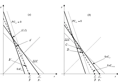
16 If (A3) does not hold, but (A4) holds, the potential homogeneous group contract is

pooling (for example, all points between A’ and B’ in fig. 2a, and between C and

D in fig. 2b are potential homogeneous pooling contracts), and we have the two following cases.

If  12, the bank’s pooling zero-profit line on homogeneous pooling contracts, )

0

( CPOOL , is closer to the zero-profit line on safe groups, (0Css), as in fig. 2a.

In this case, the cross-subsidy between borrowers is low, and safe types obtain a large expected payoff under positive matching. Mixed matching would imply a transfer so high that Uss(r,c)Usr(rMIX,cMIX)Urs(rMIX,cMIX)Urr(r,c), i.e. such

that risky types would not be able to compensate safe partners for the additional risk of default. Thus, borrowers will never choose a mixed group, and the assortative matching is positive.

If  12, (0C_POOL) is closer to the zero-profit line on risky groups, (0C_rr), as in fig. 2b. In this case, the cross-subsidy is high, and safe firms would receive a low expected return under homogeneous contracts. In particular, they would obtain a payoff close to their reservation income, and thus they may find it profitable to sell part of their risk quality to risky types. This means that the matching is negative, i.e. Uss(r,c)Usr(rMIX,cMIX)Urs(rMIX,cMIX)Urr(r,c), and

that there can be room for a Pareto improvement over positive assortative matching.

Note that the potential homogeneous pooling equilibrium depends on the relative social weight, , chosen by the MFI. For example, if 1, the homogeneous contract is at the intersection between (0CPOOL) and the binding participation constraint of safe types, (PC_ss 0), as point B’ in fig. 2a or D in fig. 2b. In this case, borrowers prefer homogeneous groups if (1’) is positive, i.e. if

0 / ) ](

1 ) 1 ( 2

[   psys u   , which is true for  12 since

0

  u 

y

17 4.1 Contract Composition

This sub-section derives the final composition of group types if the possibility of mixed matching is taken into account by the MFI.

According to Proposition 1, when (A3) holds, the potential homogeneous contract is separating, and the assortative matching can be either positive or negative. If borrowers choose homogeneous lending, in equilibrium we will observe a proportion (1)/2 of safe groups and  /2 of risky groups. On the other hand, if borrowers prefer mixed matching, we should obtain a situation in which there are min









Figure 2 – Underinvestment (potential homogeneous pooling equilibria).

a)Low θ (0C_POOLcloser to 0C_ss). b) High θ (0C_POOLcloser to 0C_rr).

r

p



LLC

D c

(a)

p

 _r

0



ss

PC

) ˆ ,ˆ (r c

LLC

c

B’

(b)

C A’

0



ss

PC

r

p



r

p



s

S

C



0

rr

C



0

POOL

C



18





max   risky groups, which receive homogeneous contracts. For the last two types of groups, the homogeneous separating equilibrium is the outcome of the classic two-stage Nash game analyzed in Section 2. On the basis of the specific combination of loan applications, the MFI will offer the corresponding number of homogeneous and mixed contracts.

When (A3) does not hold, but (A4) holds, the potential homogeneous equilibrium is pooling and we need to distinguish between two cases: a)  12; b)  12.

a)  1 2: if the proportion of risky types is low, the assortative matching is positive, so the bank will not offer the mixed contract. Again, we have (1)/2

safe groups and /2 risky groups.

b)  12: if the proportion of risky types is high, the assortative matching is negative. In equilibrium, we should have two different lending arrangements: a proportion 1 of mixed groups, which is equal to the number of safe types (the less frequent type); a proportion  of risky borrowers who cannot team up with safe types and so are forced to group homogeneously or ask for individual liability contracts.

5 Stability of the Mixed Equilibrium

This section shows that the negative assortative matching can be a stable equilibrium. To restrict the following analysis assume that, if the potential homogeneous contract is separating, the MFI chooses not to introduce the mixed contract, so that the equilibrium is as described in Section 2.

re-19 match into homogeneous pairs (safe-safe or risky-risky), under the mixed contract, (rMIX,cMIX), to further raise their payoffs with respect to true mixed pairing. Such re-matching may occur when the payoff under fake mixed groups (i.e. groups of homogeneous borrowers who sign the mixed contract) is higher than the one under true mixed lending, that is when

t c

r U c

r

Uss( MIX, MIX) sr( MIX, MIX) , or Urr(rMIX,cMIX)Urs(rMIX,cMIX)t,

where t is the ex-post transfer. Besides, the remaining risky borrowers, who cannot form mixed groups and are forced to receive homogenous group or individual loans, would obtain their full-information payoff, p_ry_r . So, they also have the incentive to form mixed groups and receive an additional payoff equal to

0 ) /(

) (

) (

) ,

( _{MIX MIX}  _{r r}   _s  _{r s} _r  _{s r} 

rr r c p y p p p p p p

U   ,

where clearly we do not have to consider any transfer between risky types within a group.

To avoid such deviations, which would make group lending unprofitable, we need to extend the reaction strategy of the MFI. This paper proposes the following four-stage game.

First stage: the bank offers a proportion of 1 mixed contracts, and 

homogeneous joint or individual contracts.

Second stage: safe borrowers randomly choose their risky partners, and apply for mixed loans. The remaining risky borrowers (who cannot form mixed groups) will either match among themselves and apply for homogeneous lending, or choose individual liability contracts.

20

Third stage: the MFI commits to withdraw the mixed contract if the number of loans is not compatible with mixed matching. If the applications for (rMIX,cMIX) are different from 1, the mixed contract is withdrawn and the bank will only offer homogeneous loans.

Fourth stage: all contracts are executed, and the game ends.

The following proposition shows that borrowers have no incentive to re-match.

Proposition 2. Under the threat of withdrawing the mixed contract, the negative assortative matching is a stable equilibrium.

Proof.

If Uss(rMIX,cMIX)Usr(rMIX,cMIX)t and Urr(rMIX,cMIX)Urs(rMIX,cMIX)t,

borrowers have no incentive to re-match.

If Uss(rMIX,cMIX)Usr(rMIX,cMIX)t and Urr(rMIX,cMIX)Urs(rMIX,cMIX)t, safe

borrowers have the incentive to re-match. If they do so, the applications for )

,

(r_MIX c_MIX would be equal to (1)/2, and the bank would withdraw the mixed contract. In this case, safe borrowers would lose the additional profit of mixed matching.

If Uss(rMIX,cMIX)Usr(rMIX,cMIX)t and Urr(rMIX,cMIX)Urs(rMIX,cMIX)t, risky

borrowers have the incentive to re-match. If they deviate, the applications for )

,

(rMIX cMIX would be  /2, and the bank would withdraw the mixed contract. In

this case, risky borrowers would lose the profits of mixed matching.

If Uss(rMIX,cMIX)Usr(rMIX,cMIX)t and Urr(rMIX,cMIX)Urs(rMIX,cMIX)t, all

borrowers have the incentive to re-match. In this case, the applications for )

,

21 should be positive for  1/2, the bank would withdraw the mixed contract, and all types would lose the profits of mixed matching.

Under the threat, the other risky borrowers, applying for homogeneous or individual loans, do not have the incentive to apply for the mixed contract (it is implicitly assumed that they have no intention to harm the other borrowers). ■

In real microcredit programs, where MFIs are usually benevolent, it is difficult to imagine that the threat described in the model should be applied in a very strict sense. In practice, it may be more reasonable to expect that, when the applications for (rMIX,cMIX) are slightly different from 1 , it can still be desirable for the MFI to promote mixed matching, although it is more exposed to losses in case of default. Probably, MFIs would face the same problem under homogeneous lending if, for some reason, borrowers were to decide to match heterogeneously (for instance, due to the presence of unobservable individual characteristics in addition to the risk quality).

Note that the MFI might use a similar withdrawing threat to encourage borrowers to accept their full-information individual liability contracts, ( ps,0) and

) 0 ,

( p_r . However, in this case, borrowers would lose the opportunity to profit from the ex-post insurance system allowed by group contracts.

22 Note also that the threat of withdrawing the contract is different from that proposed by Wilson (1977). There, the author includes a withdrawing stage to the Rothschild and Stiglitz (1976) game to prevent the cream-skimming of safe types within a perfectly competitive environment. In the present paper, the contract withdrawing is used to prevent the re-matching of borrowers who receive credit from a single benevolent MFI. In both cases, the bank can withdraw contracts that can become unprofitable, but the main difference is that the rationale for MFIs to find new and cost-effective ways to maximize the welfare of borrowers should not derive from the (short-term) profit-seeking behavior of competitive banks. Besides, in a model with a single MFI, we do not derive the coordination problem that is usually associated with the commitment mechanism of Wilson (1977), namely the ability of lenders to observe any deviation made by each other, which seems incompatible with a perfect competition framework. The possibility to change the composition of contracts can well be consistent in the context of a non-market organization, such as a large microfinance lender with some degree of monopoly power.

6 Non-existence of Homogeneous Equilibria

In the homogeneous matching equilibrium analyzed in Section 2, it is possible to observe a situation in which: 1) safe types are credit rationed under individual lending, i.e. the assumption (A2) holds, y(ps/p)u; 2) the safe project’s

expected output is at least large enough to guarantee the existence of a homogeneous pooling equilibrium, i.e. the assumption (A4) holds,

u p

p

y( s/ ) . In this case, joint liability can solve the underinvestment

problem of safe borrowers, which may arise in an individual lending scheme. On the other hand, if (A4) does not hold, the limited liability constraint is not satisfied, and no equilibrium exists under homogeneous lending. This occurs when the (LLC) is below the intersection point between the bank’s pooled break-even line, (0πCPOOL), and the binding participation constraint of safe types,

) 0

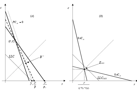
23 Similarly, if the reservation income, u, of borrowers is zero, the safe project’s output is lower than the average loan repayment, i.e. y_s /p, and homogeneous group lending is not feasible. That is, it is not possible to simultaneously satisfy assumptions (A2) and (A4). For example, in figure 3a it is

0



u , and the only candidate homogeneous equilibrium is the individual liability contract, ( p_r,0), which will only be accepted by risky types.

This section shows that, when homogeneous group lending is not possible, a mixed equilibrium may exist and solve the inefficient rationing of safe types. The condition is that the mixed limited liability constraint, (LLCMIX), must be less

stringent than (A4), i.e. that10

p p

p p u

p p p p

p s

r s r

s r

s 2

2 2

) 1 (

2   

  

 . (7)

When u0, (7) is satisfied when (1)(ps  pr pspr)/2(ps  pr), which holds for a non-empty set11 _{of values of  . And, since the right-hand side of (7) is}

increasing in u, we can state the following

Proposition 3. An equilibrium in mixed groups may exist even if homogeneous equilibria are not possible.

An example of mixed equilibrium is shown in figure 3b, where the (LLCMIX)

holds, i.e. is above the intersection between the MFI’s mixed zero-profit conditions, (0Csr) and (0Crs).

The reason why a mixed equilibrium is easier to achieve is that it hinges on ex-post payments among group members. In contrast to homogeneous group lending, in which transfers do not occur, mixed contracts allow to shift more credit risk

10 _{To ease the comparison, in (7), the assumption (A4) is rewritten in terms of}

s

y , and not of the expected profit p_sy_s  y.

11_{For example, if 0.8}

s

24 from MFIs to borrowers. This is partly confirmed by the field data in Guatemala of Wydick (2001), who reports that intra-group insurance is relevant and that this occurs through shock-contingent transfers. Thus, Proposition 3 implies that mixed lending may be a alternative instrument for MFIs to implement group lending programs in very poor environments. That is, an opportunity to better meet the needs of a fraction of potential borrowers, in particular the poorest, whose outside option is very low and who are often less likely to access credit services.

When (A4) does not hold, the homogeneous equilibrium group payoffs are as follows: safe pairs are credit rationed and obtain u; risky borrowers sign individual liability contracts and obtain the full-information payoff,

Figure 3 – Underinvestment and u0.

a) Homogeneous separating and pooling joint liability equilibria do not exist. b) Mixed pooling equilibrium.

p



0



ss

PC

) ˆ ,ˆ (r c

r p s p r p s p 



(b)

c

r EMIX

LLCMIX sr

C



0

rs

C



0

c

(a)

r

LLC _B’’

r

p



s

25

  _r  _{r r}

rr p p y

U ( ,0) ; the mixed payoffs, Usr(rMIX,cMIX) and Urs(rMIX,cMIX),

are again given by (2a) and (2b). As a result, the assortative matching expression, (1’), reduces to

0 )]

0 , ( ) , ( [ )] , (

[uU_sr r_MIX c_MIX  U_rs r_MIX c_MIX U_rr  p_r u p_sy_s  ,

which always holds under (A1). Therefore, the assortative matching is always negative and this means that, if homogeneous contracts are not available, borrowers have no choice but to form mixed groups. The reason why risky types prefer mixed matching is that they would otherwise receive the lowest possible payoff under individual liability lending, i.e. U_rr( p_r,0) p_ry_r .

7 Conclusions

The main result of this paper is that, in group lending programs, MFIs can obtain a Pareto improving solution, over positive assortative matching, by promoting a negative matching of borrowers’ types. A complementary result is that a mixed equilibrium may exist when homogeneous equilibria are not available, and thus solve the credit rationing problems that may arise under group lending.

26 APPENDIX

The Over-Investment Case

This Appendix shows that, in an environment a là de Meza and Webb (1987), the sign of the assortative matching again depends on the distribution of borrowers’ types.

Assume p_s  p_r, and ys  yr  y. Assume also that risky firms are socially

inefficient,



 u y

pr r , (A1’)

and that they nevertheless prefer to ask for outside financing, i.e. that

u p y

p_{r }

  

 

 . (A2’)

If the (LLC) is satisfied, i.e. if the assumption

   

 

 

r s p

p

y  1 1 (A3’)

holds, the homogeneous separating contract (r,ˆcˆ) exists. This means that, risky borrowers can be excluded from the credit market, and joint liability separating contracts can solve the overinvestment problem.

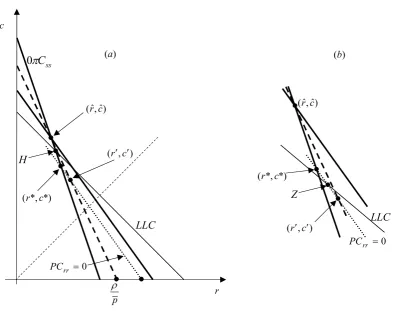
27 A.1 Homogeneous separating contracts below (r,ˆcˆ)

This type of separating contracts will depend on the extent of (LLC). Denote by

*) *,

(r c the contract at the intersection between (0Css) and (PCrr 0), and by

) ,

(r c the contract at the intersection between (0C_POOL) and (PC_rr 0), as shown, for example, in fig. 4a. The analysis can be further extended into two different subcases:

1) (LLC) on or above (r*,c*).

In this case, the separating equilibrium is at the intersection between (LLC) and )

0

( C_ss , as contract H in fig. 4a.

Figure 4 – Overinvestment (homogeneous separating equilibria).

a) LLC below (r,ˆcˆ)and above (r*,c*).

b) LLC below (r*,c*) and above (r,c)_.

p



) ˆ ,ˆ

(r c (r,ˆcˆ)

c

(a)

r

0



rr

PC

LLC ss

C



0

*) *, (r c

0



rr

PC

Z

LLC H

(b)

*) *, (r c

) , (rc

28 2) (LLC) below (r*,c*), but above (r,c).

In this case, the separating equilibrium is at the intersection between (LLC) and )

0

(PC_rr  , as contract Z in fig. 4b (which highlights a portion of fig. 4a). Note that, as in Gangopadhyay et al. (2005), the bank makes positive profits for such type of contracts, since they are above the zero-profit condition on safe types,

) 0

( C_SS .

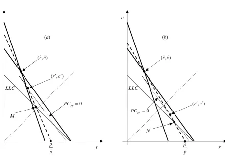
Figure 5 – Overinvestment (homogeneous pooling equilibria).

a)Low θ. b) High θ.

) ˆ ,ˆ (r c

p



c

LLC

0



rr

PC

N

) ˆ ,ˆ (r c

p



c

r LLC

0



rr

PC

M

(a) (b)

) , (r c

) , (rc

29 A.2 Homogeneous pooling contract below (r,c)

A second type of homogeneous contracts can be chosen by the MFI when (LLC) is below (r,c). See, for example, fig. 5a and fig. 5b that consider, respectively, a low and a high level of . All contracts between (r,c) and ( p,0), along

) 0

( C_POOL , are potential homogeneous pooling contracts. The set of pooling equilibria is determined by the extent of the limited liability constraint (for example, all contracts between point M and ( p,0) in fig. 5a, and between N

and ( p,0) in fig. 5b).

The condition for the existence of a homogeneous pooling equilibrium is that the project’s output in case of success must be larger than the average loan repayment,

p

y  , (A4’)

i.e. the same condition needed in an individual liability context.

A.3 Overinvestment and Assortative Matching

Assume that the MFI introduces the mixed contract, (rMIX,cMIX). Borrowers will compare the payoff received under mixed matching with that under homogeneous matching. For all potential homogeneous separating equilibria above (r,ˆcˆ), as well as for those below (r,ˆcˆ), risky types do not ask for a loan. So, we need to rewrite the assortative matching expression derived in Section 4, (1’), as

] ) , ( [ )] , ( ) , (

[Uss r c Usr rMIX cMIX  Urs rMIX cMIX u , (1’’)

30 For potential homogeneous pooling contracts below (r,c), both safe and risky types ask for a loan, so we need again the expression (1‘), and not (1’’), to compare homogeneous and mixed contracts.

Under the bank’s threat of withdrawing the mixed contract, introduced in Section 5, the composition of groups in this environment is described by the following

Proposition 4.In the overinvestment case, the assortative matching, a) if (A3’) holds, is always positive.

b) if (A3’) does not hold and (A4’) holds, is positive if  1 2, and negative otherwise.

Proof.

a) If (A3’) holds, (1’’), evaluated at (r,ˆcˆ), is equal to u pryr, which is

always positive under (A1’).

b) If (A3’) does not hold and (A4’) holds, (LLC) is below (r,ˆcˆ), and we have to consider two different possibilities:

b1) (LLC) on or above (r,c). The potential homogeneous contract is still separating. Consider first the least favorable separating contract for safe types, i.e., contract (r,c)_{. For such contract, (1’’) is positive if}

0 )

1 (

) ](

1 ) 1 ( 2

[ _

    

 

 u p_ry_{r , (8)}

which is always true for  12, since up_ry_r 0 for (A1’). Besides, given that (1’’) is increasing in Uss(r,c), (8) holds for all other possible homogeneous separating contracts between (r,c) and (r,ˆcˆ).

31 Two comments on Proposition 4 are necessary. First, if the potential homogeneous contract is separating, risky types cannot receive a homogeneous group loan, so the positive assortative matching can be interpreted as a situation where only safe groups exist. Second, the potential pooling homogeneous contract, which borrowers compare to the mixed contract, is based on the relative social weight, , chosen by the MFI. For example, if 1, the homogeneous contract is the individual liability pair ( p,0): In such a case, (1’’) reduces to

] )

1 /[( ) (

2 p_s p_r  p_s p_r p_r , so the matching is positive for 1 2.

References

Ahlin, C. (2009), ‘Matching for Credit: Risk and Diversification in Thai Microcredit Groups’, BREAD Working Paper 251.

Armendáriz de Aghion, B. and Szafarz, A. (2011), ‘On Mission Drift in Microfinance Institutions’, in Armendariz, B. and Labie, M. (Eds), The Handbook of Microfinance, London-Singapore: World Scientific Publishing.

Becker, G. S. (1973), ‘A Theory of Marriage: Part I’, Journal of Political Economy, 81, 815–846.

Berhabe, G., Gardebroek, C. and Moll, H. A. (2009), ‘Risk-matching Behavior in Microcredit Group Formation: Evidence from Northern Ethiopia’, Agricultural Economics, 40, 409–419.

Carpenter, S. and Sadoulet, L. (2000), ‘Risk-Matching in Credit Groups: Evidence from Guatemala’, Working Paper.

32 Dupas, P. and Robinson, J. (2009), ‘Savings Constraints and Microenterprise Development: Evidence from a Field Experiment in Kenya’, NBER Working Paper No. 14693.

Fafchamps, M. and Gubert, F. (2007), ‘Risk Sharing and Network Formation’,

American Economic Review, 97, 75–79.

Fafchamps, M. and La Ferrara, E. (2012), ‘Self-Help Groups and Mutual Assistance: Evidence from Urban Kenya’, Economic Development and Cultural Change, 60, 707–733.

Gangopadhyay, J. E., Ghatak, M. and Lensink, R. (2005), ‘Joint Liability Lending and the Peer Selection Effect’, Economic Journal, 115, 1005–1015.

Ghatak, M. (1999), ‘Group Lending, Local Information and Peer Selection’,

Journal of Development Economics, 60, 27–50.

Ghatak, M. (2000), ‘Screening by the Company You Keep: Joint Liability Lending and the Peer Selection Effect’, Economic Journal, 110, 601–631.

Guttman, J. M. (2008), ‘Assortative Matching, Adverse Selection, and Group Lending’, Journal of Development Economics, 87, 51–56.

Kremer, M. and Maskin, E. (1996). ‘Wage Inequality and Segregation by Skills’,

National Bureau of Research Working Paper Series W5718.

Lensik R. and Mehrteab, H. T. (2003), ‘Risk Behavior and Group Formation in Microcredit Groups in Eritrea’, Working Paper.

Navajas, S., Schreiner, M., Meyer, L. R., Gonzalez-Vega, C. and Rodriguez-Meza, J. (2000), ‘Microcredit and the Poorest of the Poor: Theory and Evidence from Bolivia’, World Development, 28, 333–346.

33 Roy Chowdhury, P. (2007), ‘Group-lending with Sequential Financing, Contingent Renewal and Social Capital’, Journal of Development Economics, 84, 487–506.

Sadoulet, L. (1999), ’Equilibrium Risk-Matching in Group Lending’, Working Paper.

Stiglitz, J. E. (1990), ‘Peer Monitoring and Credit Markets’, World Bank Economic Review, 4, 351–366.

Stiglitz, J. E. and Weiss, A. (1981), ‘Credit Rationing in Markets with Imperfect Information’, American Economic Review, 71, 393–410.

Topkis, D. M. (1998), ‘Supermodularity and Complementarity’, Princeton University Press.

Van Tassel, E. (1999), ‘Group Lending Under Asymmetric Information’, Journal of Development Economics, 60, 3–25.

Van Tassel, E. (2000), ‘A Study of Group Lending Incentives in Bolivia’,

International Journal of Social Economics, 27, 927–942.

Vigenina, D. and Kritikos, A. S. (2004), ‘The Individual Micro-lending Contract: Is It a Better Design than Joint-liability?: Evidence from Georgia’, Economic Systems, 28, 155–176.

Wilson, C., (1977), ‘A Model of Insurance Markets with Incomplete Information’,

Journal of Economic Theory, 16, 167–207.