Munich Personal RePEc Archive
Social Motives vs Social Influence: an
Experiment on Time Preferences
Rodriguez-Lara, Ismael and Ponti, Giovanni
1 February 2017
Online at
https://mpra.ub.uni-muenchen.de/76486/
Social Motives
vs
Social Influence:
an Experiment on Time Preferences
∗
Ismael Rodriguez-Lara
Middlesex University London
Giovanni Ponti
†Universidad de Alicante, University of Chicago
and LUISS Guido Carli Roma
Abstract
We report experimental evidence on the effects of social preferences on intertemporal decisions. To this aim,
we design anintertemporal Dictator Game to test whether Dictators modify their discounting behavior when
their own decision is imposed on their matched Recipients. We run four different treatments to identify the
effect of payoffs externalities from those related to information and beliefs. Our descriptive statistics show that
heterogeneous social time preferences and information about others’ time preferences are significant determinants
of choices: Dictators display a marked propensity to account for the intertemporal preferences of Recipients,both
in the presence of externalities (social motives) and/or when they know about the decisions of their matched
partners (social influence). We also perform a structural estimation exercise to control for heterogeneity in risk
attitudes. As for individual behavior, our estimates confirm previous studies in that high risk aversion is associated
with low discounting. As for social behavior, we find that social motives outweigh social influence, especially when
we restrict our sample to pairs of Dictators and Recipients who satisfy minimal consistency conditions.
Keywords: intertemporal choices, time preferences, risk and social preferences, social influence, beliefs.
JEL Classification: C91, D70, D81, D91.
∗We thank Daniel M¨uller, Vincent Crawford and two anonymous referees for their useful comments and suggestions, which
improved the quality of the manuscript significantly. We also thank seminar participants at the European University Institute,
the 2013 IMEBE Meeting (Madrid), SEET (Tenerife), the PET Meeting 13 (Lisbon), the Alhambra Meets Colosseo AEW
Meeting (Rome), the I London Experimental Workshop, and the FUR 2014 Meeting (Rotterdam). This paper has been revised
while Giovanni Ponti was visiting the Center for Experimental Social Science (CESS) at New York University. He would like
to thank Alberto Bisin, Guillaume Fr´echette, Alessandro Lizzeri, Caroline Madden, Andrew Schotter and all people at CESS
and Econ NYU for their kind hospitality. Finally, a special thank goes to Daniela Di Cagno, who has been involved in the
earlier developments of this project. The usual disclaimers apply. Financial support from the Spanish Ministry of Economy
and Competitiveness (ECO2014-58297-R and ECO2015-65820-P), Generalitat Valenciana (Research Projects Grupos 3/086)
and Instituto Valenciano de Investigaciones Econ´omicas (IVIE) is gratefully acknowledged.
†Corresponding author. Departamento de Fundamentos del An´alisis Econ´omico, Universidad de Alicante 03071 Alicante
“At the first time of sexual union the passion of the male is intense, and his time is short [...]
With the female, however, it is the contrary, for at the first time her passion is weak, and then her time long [...]
If a male be a long-timed, the female loves him the more, but if he be short-timed, she is dissatisfied with him.”
“The Kama Sutra of Vatsyayana” - Burtonet al. [19]
1
Introduction
We often show concerns for others by changing the timing of a specific course of action. This happens
routinely in household key decisions such as selling a house, investing in a pension plan or even getting
divorced. The empirical literature on health economics has extensively studied the relationship between time
preferences for one’s own private health and for others’ health (see Lazaro et al. [53], [54] or Robberstad [63] for earlier contributions on this area and Mahboub-Ahariet al. [55] for a recent meta-analysis). It is also well documented (see, e.g., Abdellaouiet al. [1], Browning [17], Mazzocco [56], [57], among others) that multi-person household saving and consumption patterns may strongly differ from those of single-person
households, even after controlling for individual characteristics (e.g., own risk aversion, or discounting) of
each household component. As all these examples illustrate, social (i.e., interdependent) concerns may affect the timing of choices: decision makers may try to accommodate others’ intertemporal concerns, when
decisions affect the latter’s prospects and welfare.
This paper aims at providing evidence on the effects of social preferences on intertemporal decisions. More in detail, we are interested in better understanding how much -and in which direction- individuals’
preferences for anticipating or delaying an action can be affected by the presence of payoff externalities.
Clearly, our motivating examples lead to a broader concept of social preferences, compared with its current
usage in the flourishing -mainly experimental- literature on these matters, where social preferences are usually
restricted to people’s interest on “the fairness of their own material payoff relative to the payoff of others...” (Fehr and Schmidt [30], p. 819). In contrast with this literature, in this paper concerns for others may
not only involve others’ material consequences (e.g., monetary outcomes, consumption bundles), but also others’concerns and inclinations, such as risk aversion or discounting. This, in turn, calls for modeling social preferencesas mapped directly on others’ individual utilities (Harrisonet al. [42]).
is, probably, the reason why the mainstream literature has always preferred to restrict the domain of social
preferences to the physical outcome space). By contrast, the empirical literature we just cited -take, e.g.
Mazzocco [57], eq. (3)- posits that households maximize a convex linear combination of the individual
(“self-ish”) utilities of their members, which are assumed to be derived as different parametrizations -depending on
individual characteristics- of the same functional, with weights being interpreted as proxies of each member’s
bargaining power within the household. This is going to be the modeling approach we use in this paper.
Our empirical evidence comes from a multi-stage laboratory experiment where we investigate on the link
between time and social preferences by way of Multiple Price Lists (MPLs, Holt and Laury [46], [47]). Since
time and risk preferences are interwined, we follow Andersen et al. [5] by eliciting (own) risk and time preferences by way of separate tasks in the first two stages of the experiment (see also Andersenet al. [6], Harrisonet al. [39], [40] or Sutteret al. [67] for applications of similar methods). Thus, we use MPLs to elicit risk preferences and control for the curvature of subjects’ utility function when estimating time preferences
by way of another sequence of ten MPLs in which subjects are asked to choose between an immediate smaller
reward and an increasingly larger later reward. The novelty of our approach relies on incorporating asocial dimension to this protocol. Thus, once subjects have completed the first two stages, we match them in pairs and randomly assign the roles of Dictators and Recipients. Then, Dictators go through, once again, the same sequence of intertemporal decisions knowing that -this time- their choices may also be implemented for
their assigned Recipient. Subjects’ information on others’ risk and time decisions and the presence of payoff
externalities defines our treatment conditions:
1. in the baseline treatment (T0, INFO-SOCIAL), Dictators make their intertemporal choices after being
informed of what their assigned Recipient had chosen in the first two stages of the experiment;
2. in the BELIEF-SOCIAL treatment (T1), before deciding for the pair, Dictators go through an additional
stage in which we elicit their beliefs on risk and time concerns of their assigned Recipient;
3. in the INFO-PRIVATE treatment (T2), subjects receive (exactly as in the baseline) information on
risk/time individual choices of their groupmate, but no payoff externalities are imposed on others;
4. in the NO INFO-SOCIAL treatment (T3), Dictators make their intertemporal decisions for the pair
without prior knowledge (or elicited belief) of the Recipient’s risk/time decisions.
Our design strategy allows to tease apartsocial motives fromsocial influence. The comparison between the INFO-SOCIAL and the INFO-PRIVATE treatments allows us to determine whether informed Dictators
situation in which -whatever the reason- they can just mimic the behavior of their assigned Recipient (social
influence), without imposing any payoff consequence on the latter.1 Along similar lines, we can also compare
the behavior of uninformed Dictators in the BELIEF-SOCIAL and the NO INFO- SOCIAL treatments so
as to measure the impact of belief elicitation in the emergence of social (time) preferences. This is what
Krupka and Weber [51] label as the effect offocusing on social preferences: guessing and thinking about the actions of others leads -in standard Dictator games- to focus more on the social norm and, as a result, more
generosity is observed.
Following Rodriguez-Lara [64], our experimental design is built around the structural estimation exercise
of Section 4.2, in which subjects’ behavior is framed by way of a convex linear combination between the
(“selfish”) utilities of Dictator and Recipient. By contrast with the literature cited earlier, here weights
reflect the Dictator’s concerns about the Recipient’s risk aversion and discounting. In this respect, our
identification strategy crucially relies on the experimental design by manipulating subjects’ incentives and
information in the various stages of the experiment.
The remainder of the paper is arranged as follows. Section 2 reviews the relevant literature on these
matters. In Section 3 we lay out our experimental design, whereas Section 4 reports our results. First,
Section 4.1 reports some descriptive statistics on subjects’ behavior in the various stages of the experiment.
Here we show that i) Dictators’ choices significantly move in the direction of their matched Recipients in
our basline treatment;ii) social influence is another important factor in explaining choices, in that Dictators
tend to move in the direction of Recipients also in the INFO-PRIVATE treatment and iii) Krupka and
Weber’s [51] focusing effect is also relevant in the absence of information in that eliciting beliefs seems to trigger social preferences in the BELIEF-SOCIAL, compared with the NO INFO-SOCIAL treatment.
Section 4.2 tests the robustness of our preliminary findings by way of a structural model in which we
frame subjects’ choices within the realm of a random utility maximization problem, by which we can control
for subjects’ heterogeneity in risk preferences. We look both at subjects’i)individual decisions (and elicited beliefs) in Stages 1 to 3, as well as ii) Dictators’ intertemporal choices in Stage 4. As for the former, our evidence is consistent with previous findings in that our subjects exhibit, on average, (Constant Relative)
Risk Aversion (CRRA, Hey and Orme [45], Holt and Laury [46]) and non-exponential discounting (Colleret al. [24], Benhabibet al. [14], Andersenet al. [5]). In addition, we also find (consistently with Sutter et al.
1
The role of social influence was first studied in Psychology by Sherif [65] and Asch [12]. The economic literature on this topic
includes papers oninformational influence, that is, herding or observational cascades (see, e.g., Banerjee [13], Bikhchandaniet
al. [16] or Feriet al. [31]) andnormative influence, that is, imitation based on moral judgement (see, e.g., Hung and Plott
[48] or Moreno and Ramos-Sosa [60]). The interested reader on the comparison between these two behavioral phenomena can
[67] and Dean and Ortoleva [27]), that individual (own) risk and time preferences are strongly correlated,
in that risk averse subjects are also more patient. Finally, we see that -once we control for risk aversion in
our structural estimation- social motives outweigh both social influence and focusing, in that the estimated
weight of the Recipient’s utility is positive and highly significant only when externalities and information
are both present (i.e., in our baseline treatment). By contrast, the “social influence” conjecture (proxied by the estimated weight for the INFO-PRIVATE treatment) is only partially validated, since the estimated
coefficient remains positive, but is only significant at 10% confidence, and only when we do not restrict our
sample to pairs of Dictators and Recipients who satisfy minimalconsistency conditions (see Section 4.1.3). Also for the focusing hypothesis, the estimated weight in the BELIEF-SOCIAL treatment is positive, but
not significant.
Finally, Section 5 concludes, followed by Appendices containing information on the identification strategy,
the experimental instructions, the debriefing questionnaire and supplementary experimental evidence.
2
Related literature
Notwithstanding our “social twist”, this paper sits squarely in the emerging literature that applies
experi-mental methods to study the link between individual risk and time preferences (see, among others, Andreoni
and Sprenger [10], [11], Halevy [38], Laury et al. [52]). In this respect, we borrow the methodology put forward by Andersenet al. [5] and control for the curvature of the utility function when eliciting discount rates. To this aim, a double MPL is employed to elicit risk and time preferences independently, that is, with two separate tasks: one MPL over lotteries paid off at the time of the experiment (Stage 1), another
intertemporal MPL of certain monetary payoffs paid off at different times (Stage 2). Similar methods have
been employed by Andersenet al. [4], [6], Harrisonet al. [40], Cheung [22], Sutteret al. [67] or Frederick et al. [34], among others.
Andreoni and Sprenger [11], instead, apply an identification strategy between risk and time preferences
in which subjects allocate a budget of tokens between risky prospects that reward at different points in time
(see also Miao and Zhong [59]). With this design, the null hypothesis of risk neutrality is also rejected.
Other methods to elicit time preferences are those of Benhabibet al. [14], where subjects are asked to elicit intertemporal equivalents, i.e., the amount of money that received today (in the future) that would make them indifferent to some amount paid in the future (today) or Lauryet al. [52], where the elicitation of risk preferences does not require any assumption on the form of the utility function.2
2
Along similar lines, we here mention an emerging literature that, by way of joint elicitation of risk and
social preferences, claims that the empirical content of the latter may be severely reduced by the presence
of some -strategic, or environmental- uncertainty (Winteret al. [69], [70], Cabraleset al. [20], Frignani and Ponti [35]).3
To the best of our knowledge, this is the first paper that elicits discount rates in a model of social
preferences. The only related precedents we are aware of are the papers of Phelps and Pollack [61] and
Kovarik [50]. Phelps and Pollack [61] propose an intergenerational model in which each generation cares
about the consumption of future generations, which is discounted in a non-linear manner. Kovarik [50]
collects evidence on the relationship between altruism and discounting, showing that donations in a Dictator
Game decrease as the moment for receiving payments is delayed. This contradicts standard theories of time
preferences, including exponential and hyperbolic discounting.
Last, but not least, given that our estimation strategy involves the joint elicitation of risk, time and social
preferences by way of separate experimental tasks, our findings are to be compared with those of some recent
papers that establish empirical correlations among these behavioral traits. In this respect, our finding are
consistent with those of Sutteret al. [67], in thatsubjects with a comparatively lower degree of risk aversion discount the future significantly more (see also Burks et al. [18] and Dean and Ortoleva [27]). Because our debriefing questionnaire collects a wide variety of individual characteristics, we can also establish a positive
correlation between the willingness to accept the delayed payment and the score in the cognitive skills, also
reported by Andersonet al. [7] or Burkset al. [18].4
3
Experimental design
3.1
Sessions
Thirteen experimental sessions were run at the Laboratory for Research in Experimental Economics
(LI-NEEX), at the Universidad de Valencia. A total of 624 subjects (48 per session) were recruited within the
undergraduate population of the University. The experimental sessions were computerized. Instructions
were read aloud and we let subjects ask about any doubt they may have had. All sessions ended with a
debriefing questionnaire to distill subjects’ individual socio-demographics and social attitudes.5 Each session
3
Anderssonet al. [8], Chakravartyet al. [21] and Harrisonet al. [41] are further examples of the investigation of social
preferences in the risk dimension.
4
See Appendix D2.
5
The experiment was programmed and conducted with the softwarez-tree (Fischbacher [32]). Translated versions of the
lasted, on average, 1 hour and 40 minutes.
3.2
Stages
Each subject participates to one of the four treatment conditions (T0 to T3). Stages 1 and 2 (common to
all treatments) are used to elicit individual (own) risk and time preferences, respectively. After Stage 2,
participants are matched in pairs. In one of the treatments (T1, labeled as BELIEF-SOCIAL), subjects face
an additional stage (Stage 3) in which we elicit their beliefs on (own) risk and time preferences of their
assigned groupmate. Then, in Stage 4 (common to all treatments), we assign subjects the role of Dictator
and Recipient, and all subjects go again through the same sequence of decisions of Stage 2. Our treatment
conditions (Section 3.6) determine whether the Dictators’ decision in Stage 4 is binding for the Recipient,
and the information Dictators receive (if any) about the Recipients’ decisions in Stages 1 and 2.
3.3
Stage 1. Own risk preference elicitation
We elicit subjects’ individual risk preferences by way of a MPL in which subjects face the ordered array
of binary lotteries of Figure 1. As Figure 1 shows, subjects face a sequence of 11 binary lotteries, one for
each row. The entire sequence is characterized by the fact that the “risky” option (B) is increasingly more
profitable, as the probability of the highest prize (e190, in our parametrization) grows in probability, and so
is falling the expected payoff difference between options A and B. In decision 1 (11) lotteries are degenerate,
giving probability 1 to the lower (larger) prize for lottery A and B, respectively. A risk-neutral subject
should be switching from option A to B in decision 6, when the expected payoff difference between option
A and option B goes negative. The higher the switching point, the more risk averse the subject is.
3.4
Stage 2. Individual time preference elicitation
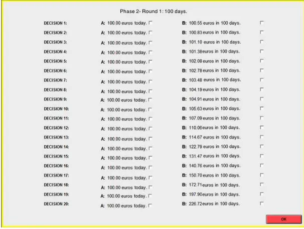
MPLs are also used to elicit time preferences. In Stage 2 subjects go through 10 decision rounds, each of
which is characterized by a specific time delay,τ, ranging from 1 to 180 days. For each MPL,τ, subjects face
20 binary choices,k, and choose between receivinge100 in the day of the experiment (hereafter ”today”)
and e100 (1 + ik 365)τ
in τ days, where the sequence of Annual Interest Rates (AIR),ik, constant across
rounds, τ, varies from 2% to 300%. Delays correspond to τ = 1,3,5,7,15,30,60,90,120 and 180 days.
Figure 2 reports the user interface of the MPL corresponding to a delay of 100 days, the same used in the
experimental instructions.6 Contrary to other studies (e.g., Andersenet al. [5] [6], Coller and Williams [23],
6
Figure 1: Stage 1 user interface
Colleret al. [24]) the AIR is not shown to subjects in the user interface. Another important difference with respect to these papers is that subjects do not make a unique intertemporal decision (with different delays
distributed between subjects). Instead,all subjects go through all intertemporal MPLs.7
Contrary to what happens in Stage 1, subjects make only one decision for MPL, in that they are
simply asked to indicate their “switching point” (if any) from option A (e 100 “today”) to option B (e
100 (1 +yk) τ
365 inτ days). Thus, “time consistency” (see Section 4.1.3) within each MPL -but not across
MPLs- is artificially imposed.
3.5
Stage 3. Belief elicitation (only for
T
1)
As we explained earlier, at the end of Stage 2 subjects are matched in pairs. In one of our treatments,
(T1, BELIEF-SOCIAL) subjects are asked to predict their matched partner’s decisions in Stages 1 and 2.
Predictions are incentivized, as detailed in Section 3.8.
7
Figure 2: Stage 2 user interface
3.6
Stage 4. Social time preference elicitation
In Stage 4, for each matched pair, subjects are assigned the role of Dictator or Recipient (with the exception
of T2, where all subjects can be considered as “Dictators” of their own fate). All subjects are reminded
about their own choices in Stages 1 and 2. Then, both Dictators and Recipients go through -once again- the
same sequence of MPLs as in Stage 2.8 Subjects’ information on others’ risk and time preferences -together
with the presence of payoff externalities- define our treatment conditions, as follows:
• In our baseline treatment (T0, INFO-SOCIAL: 6 sessions, 288 subjects), Dictators are informed about
their partner’s choices in Stages 1 and 2 before making their decision for the pair.
• In the BELIEF-SOCIAL treatment (T1: 2 sessions, 96 subjects) Dictators are reminded about their
own predictions of Stage 3 before making their decision for the pair. As inT0, the Dictator’s decision
has payoff consequences for the pair in that the Dictator’s choice imposes a payoff externality on the
Recipient.
8
Also Recipients go through the same sequence of decisions, although it is made clear in the instructions that Recipients’
• In the INFO-PRIVATE treatment (T2: 3 sessions, 144 subjects), all subjects receive information about
the decision of their matched partner in Stages 1 and 2 exactly as inT0, but no payoff externalities are
imposed. Thus, all subjects choose again across all 10 decision rounds, τ, the payoff they would like
to receive for themselves (as in Stage 2).
• In the NO-INFO-SOCIAL treatment (T3: 2 sessions, 96 subjects), neither Dictators receive information
about the Recipients’ previous decisions, nor we elicit the Dictators’ beliefs about Recipients’ behavior
in Stages 1 and 2. By analogy with treatmentsT0andT1, Dictators’ decisions have payoff consequences
for their matched Recipients.
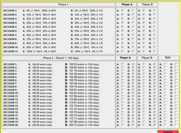
Figure 3 reports the Stage 4 user interface for our baseline treatment (INFO-SOCIAL). As Figure 3
shows, the top (bottom) screen provides information about the lottery (intertemporal) choices of Stage 1
and 2, for both the deciding subject (Player A) and her assigned partner (Player B), where the information
about the latter refers to the Recipient’s actual choice (or the Dictator’s elicited belief) depending on the
treatment condition. In the NO INFO-SOCIAL (T3) treatment the Player B column is hidden, in that
Dictators make a decision for the pair without any information on the Recipients’ decisions in Stages 1 and
[image:11.612.154.458.450.673.2]2.
3.7
Matching
Along the development of this research project, three are the matching protocols that have been used.
1. Random Matching (RM). In this case, Dictators and Recipients are randomly matched, with no further restriction.
2. Dissortative Matching (DM). In this case, we use data from Stage 2 to compute the average switching point per subject across all 10 decision rounds,τ, where average switching point is taken as a proxy of
individual discounting (the higher the switching point, the lower the discounting). We then match the
most patient Dictator with the most impatient Recipient, the second most patient Dictator with the
second most impatient Recipient, and so on. This design feature makes that Dictators are the most
patient subjects in half of the couples, to provide sufficient dispersion/variability in the data minimize
the possibility of matchings between subjects with very similar time preferences, thus making social
preferences very difficult to identify.
3. Efficient Random Matching (ERM). In this case, we impose that consistent Dictators are randomly matched with consistent Recipients whenever possible. This design enhances efficiency of our structural
estimation exercise (see Section 4.1.3).9
Table 1 summarizes our treatment layout, including information on the number of sessions (by matching
[image:12.612.71.555.519.632.2]protocol) and the number of subjects (Dictators) in each of the treatments.
Table 1: Treatment conditions
Cod. Treat. Info Pay. Ext. #Sessions (RM/DM/ERM) #Subj. (Dict.)
T0 INFO-SOCIAL Yes Yes 6 (1/ 2/ 3) 288 (144)
T1 BELIEF-SOCIAL Beliefs Yes 2 (2/ 0/ 0) 96 (48)
T2 INFO-PRIVATE Yes No 3 (1/ 1/ 1) 144 (144)
T3 NO INFO-SOCIAL No Yes 2 (2/ 0/ 0) 96 (48)
Total 13 (6/ 3/ 4) 624 (384)
9
We are grateful to two anonymous referees for expanding the scope of the paper and considering alternative matching
3.8
Financial rewards
All subjects receive e 10 just to show up. For the payment of Stages 1 and 2, we select at random one
subject and one decision per session for payoff. By analogy, in Stage 3 we randomly pick one subject and
one Stage 1or Stage 2 prediction. A prize ofe100 is paid in case of a correct guess.10 As for Stage 4, we follow the same payment protocol as in Stage 2: one matched pair and one decision is selected at random
and both, the Dictator and the Recipient, are paid according to the Dictator’s choice.
All choices are paid at the end of the experiment, when we randomly select 2 subjects per stage for
the payment of a randomly selected decision.11 The show-up fee and the decisions for Stages 1 and 3 are
paid in cash on the same day of the experiment. By contrast, we take extreme care with the payment of
Stages 2 and 4, as we are concerned with the transaction costs associated with receiving delayed payments
(including physical costs and payment risk). To make all choices equivalent except for the timing dimension,
all payments are made by way of a bank transfer to the subjects’ account. This is to minimize transaction
costs and equalize them across periods, including payments for subjects who opt for the payment “today”.12
The dates of all delayed payments were set to avoid public holidays and weekends.
3.9
Debriefing
All sessions end with a (computerized) debriefing questionnaire including, among others,
1. standard socio-demographics, such asgender, a dummy variable positive for female; the rooms/household size ratio,RSR, a standard proxy of the household wealth, together with the self-reported weekly
bud-get,WB;
2. proxies of cognitive ability, such as Frederick’s [33] Cognitive Reflection Test (CRT), a 3-item task of quantitative nature designed to measure the tendency to override an intuitive and spontaneous response
alternative that is incorrect and to engage in further reflection that leads to the correct response;
10
This, in turn, implies that our belief elicitation protocol is neutral to subjects’ degree of risk aversion (see Andersenet al.
[3]).
11
Although this method yields a compound lottery over the various stage decisions, there exists substantial evidence showing
that this does not create a response bias (see, among others, Starmer and Sugden [66], Cubittet al.[25] and Hey and Lee [44]).
12
We run all sessions at 10 a.m. to ensure that subjects would receive the bank transfer the same day of the experiment if
this was selected for payment. To control for credibility in the payment method, we add a formal legal contract between the
legal representative of the laboratory (LINEEX) and the subjects who were selected for payment. This contract is privately
received by the subjects in an envelop and includes a formal statement on a 20% compensation if payments do not take place
3. proxies of social capital drawn from theWorld Values Survey, such as self-reported measures of indi-vidual happyness, or personal inclinations toward trust(see Glaeser et al. [36]) andinequality.
4
Results
Section 4.1 provides summary statistics of our behavioral data, stage by stage, while in Section 4.2 we
perform a structural estimation exercise, where subjects’ risk, time and social preferences are framed within
the realm of a parametric welfare function consisting in a convex linear combination between the Dictator’s
and the Recipient’s “selfish” utilities. Section 4.1.3 includes a discussion on the consistency of choices and
how it affects our structural estimations.
4.1
Descriptive statistics
4.1.1 Stages 1 and 3: risk preferences
Figure 4 plots the relative frequencies of subjects selecting the “safe” option (A) across all 11 lotteries in
Stage 1 (all treatments) and Stage 3 (treatment BELIEF-SOCIAL). Figure 4 also reports optimal choices
under Risk Neutrality (RN), which correspond to the lottery with the highest expected value (i.e., Option
A in the first 5 decisions and Option B thereafter).13
As Figure 4 shows, subjects display aggregate risk aversion, in that switching to Option B occurs at a
slower pace, compared with the RN benchmark (p <0.001).14 As expected, we do not detect any significant
treatment conditions using the Krusall-Wallis test (p= 0.148).
4.1.2 Stages 2 and 3: individual time preferences
Remember that, for each of the 10 delays,τ, subjects must identify the minimum amount of money (if any)
they would need to receive in the future against the immediate bank transfer ofe100. Figure 5 summarizes
subjects’ behavior in stages 2 (all treatments) and 3 (treatmentT1), with the vertical axis representing the
distribution of “average switching points”, that is, the first decision (out of a sequence of 20) for which
subjects express their preference for the delayed payment.15
13
Figure D1 in Appendix D reports the same information by matching protocol.
14
Unless otherwise stated, all reportedp-values are derived from a (two-tail) Wilcoxon-Mann Whitney test between-subject
and a Wilcoxon signed-rank test within-subject.
15
If a subject always prefers the immediate payment, we assign this choice with “option 21”, which is also averaged out in
Figure 4: Aggregate behavior in the lottery tasks
[image:15.612.166.452.438.646.2]As Figure 5 shows, average switching points decrease with delay (i.e., for increasing delays, subjects’
indifference interest rate goes down). This evidence contradicts (is consistent with) exponential (hyperbolic)
discounting, respectively.
4.1.3 Inconsistent behavior
To the extent to which, in the structural estimations of Section 4.2, we frame subjects’ behavior within
the realm of specific parametric models (along with all the implicit auxiliary assumptions that come with
them), we are interested in a prior check on whether observed behavior satisfies basicconsistency conditions compatible with our postulated theoretical setup.
In the MPL of Stage 1, standard behavioral restrictions (namely, monotonicity, first-order stochastic
dominance and transitivity) require that subjects who face the MPL of Stage 1 satisfy the following
Condition 1 A subject should choose option A in the first row, option B in the last row, and switch from option A to B once -and once only- along the sequence.
We also look along similar lines at the intertemporal decisions of Stage 2. Remember that we force
subjects to switch at most once within each MPL, i.e., consistency is artificially imposed within delays, τ, by the same experimental design. No further restriction is imposed by the experimental protocol when
comparing choicesacross MPLs. In this respect, a natural requirement is contained in the following
Condition 2 If a subject preferse100 today against any higher amountexat some pointτ in the future,
then, for allτ′ > τ, she should never preferex′< x against e100 today.16
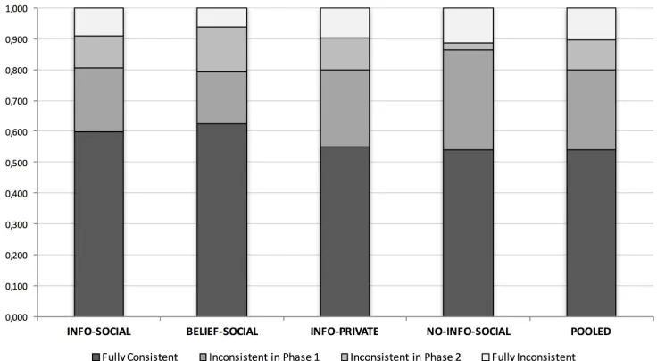
Figure 6 reports an overview of our data with regard to inconsistent behavior, as defined by both
con-ditions 1 and 2. We consider four different categories, depending on whether subjects are in/consistent in
the risk (Condition 1) and/or the time preference (Condition 2) task. As Figure 6 shows, roughly 60% of
our pool (352 subjects out of 624) passes both our consistency tests, and we cannot reject the null that the
distribution of in/consistent subjects is the same across treatments (Krusall-Wallis test, two-tail: p=0.98).
Motivated by the evidence of Figure 6, we are interested in characterizing subjects’ inconsistency by way
of the observable heterogeneity that can be inferred by the debriefing questionnaire. To this aim, we first
partition our subject pool in four groups, depending on their risk (intertemporal) in/consistency, respectively.
Since our two proxies of consistency are strongly correlated (Spearman Beta=0.17,p <0.01), Table 2 reports
the estimates ofi)the probability of being inconsistent in either task by way of a bivariate probit regression,
16
Figure 6: In/consistent behavior in Stages 1 and 2
where the set of covariates includes proxies from the questionnaire andii)the probability of failing at least one of our consistency tests (incDUMMY) against the same set of covariates by way of a standard logit
regression.17 As it turns out, both genderand CRT play a key role in our estimations. This is why we
include in the regressions an interaction term, and also report our estimations by gender.
Our findings suggest a positive (negative) significant effect of gender(CRT) on the likelihood of
incon-sistent behaviour in any of the two stages, as both marginal effects are highly significant. When we condition
our estimates on gender, we observe thatCRThas a significant (negative) effect, but only for females. By
contrast, socio-demographics or social capital proxies have only a marginal impact in all regressions. This is
consistent with previous results in the literature (take, e.g., Frederick [33] and Cuevaet al. [26]).18
Once we have acquired a better grasp on the main determinants of inconsistent behavior, the next –rather
delicate– question is what to do with those subjects who do not pass our consistency tests. This is because
our behavioral paradigm –with specific reference to the structural estimations of Section 4.2– imposes much
17
The reported marginal effects follow the approach put forward by Ai and Norton [2] and Karaca−Mandicet al. [49] in the
estimation of marginal effects in nonlinear models that include interaction terms. We also run a probit regression (not reported
here) with qualitatively similar results.
18
The interested reader on the effects of cognitive reflection and gender in intertemporal preferences can look, among others,
Table 2: In/consistent behavior: regression results
Notes. Standard errors in parentheses *** p<0.01, ** p<0.05, * p<0.1
Inconsistent (Pooled Data) Inconsistent (Males) Inconsistent (Females) Stage 1 Stage 2 incDUMMY Stage 1 Stage 2 incDUMMY Stage 1 Stage 2 incDUMMY
Logit estimates
Gender (=1 if women) 0.602*** 0.313** 0.905***
(0.137) (0.148) (0.215)
Cognitive reflection (CRT) -1.022*** -0.033 -0.901* -1.015*** 0.009 -0.903* -1.719*** -1.509*** -3.043*** (0.343) (0.322) (0.486) (0.341) (0.316) (0.488) (0.358) (0.407) (0.594)
Interaction (Gender x CRT) -0.654 -1.430*** -2.134***
(0.490) (0.522) (0.767)
Weekly Budget 0.002* 0.002* 0.004** 0.002 -0.001 0.004 0.002 0.005*** 0.004
(0.001) (0.001) (0.002) (0.002) (0.002) (0.003) (0.002) (0.002) (0.003)
Room Size Ratio 0.158 0.175* 0.288* 0.102 0.151 0.322 0.194 0.226* 0.247
(0.098) (0.093) (0.171) (0.148) (0.145) (0.264) (0.139) (0.122) (0.222)
Happiness -0.834*** -0.159 -1.013*** -0.640** -0.407 -0.907* -0.964*** 0.015 -1.088** (0.218) (0.216) (0.339) (0.323) (0.329) (0.486) (0.293) (0.294) (0.478)
Trust (General Social Survey) -0.494** 0.047 -0.339 -0.176 0.325 -0.069 -0.696** -0.065 -0.555
(0.236) (0.274) (0.375) (0.368) (0.438) (0.567) (0.309) (0.361) (0.507)
Inequality Loving -0.861** -0.041 -0.844 -0.318 0.410 -0.262 -1.198** -0.240 -1.288
(0.415) (0.484) (0.663) (0.663) (0.815) (1.051) (0.537) (0.607) (0.873)
Constant 0.410 -1.174** 0.263 -0.141 -1.261* -0.317 1.367*** -0.964 1.637** (0.388) (0.475) (0.636) (0.580) (0.761) (0.951) (0.509) (0.590) (0.833)
Marginal Effects
Gender 0.392*** 0.184*** 0.470***
(0.028) (0.024) (0.029) Cognitive reflection (CRT) -0.466*** -0.241*** -0.495***
(0.079) (0.083) (0.077)
Obs. 624 624 624 277 277 277 347 347 347
stronger consistency conditions, whose violation may affect our numerical exercise in unexpected directions,
whose interpretation goes well beyond the scope of this paper. In this respect, our analysis of individual
behavior in Stages 1 to 3 (sections 4.1.4 and 4.2.1) follows the approach in Dean and Ortoleva [27] or Sutter
et al. [67] in that we discard all observations from inconsistent subjects. This reduces our database to 352 subjects out of 624 (56%). As for the analysis of Dictators’ choices in Stage 4 (sections 4.1.4 and 4.2.2), we
focus the analysis on those consistent Dictators who satisfy Conditions 1 and 2. This reduces our database
to 210 subjects out of 384 (53%). As some of these consistent Dictators might have received information
about inconsistent Recipients in the INFO-SOCIAL and the INFO-PRIVATE treatments, we control for the
inconsistency of Recipients in the regressions of Table 6. Along similar lines, in our structural estimations
we also check whether Dictators’ beliefs in treatment T1 satisfy the same consistency conditions. Table 3
summarizes the number of in/consistent pairs in each treatment. This includes information about consistent
beliefs in treatment T1 and consistent Dictators in the NO INFO-SOCIAL treatment, where Dictators
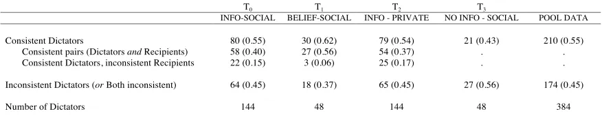
[image:18.612.88.527.165.428.2]Table 3: Number of in/consistent pairs in each treatment
T0 T1 T2 T3
INFO-SOCIAL BELIEF-SOCIAL INFO - PRIVATE NO INFO - SOCIAL POOL DATA
Consistent Dictators 80 (0.55) 30 (0.62) 79 (0.54) 21 (0.43) 210 (0.55) Consistent pairs (Dictators and Recipients) 58 (0.40) 27 (0.56) 54 (0.37) . . Consistent Dictators, inconsistentRecipients 22 (0.15) 3 (0.06) 25 (0.17) . . Inconsistent Dictators (or Both inconsistent) 64 (0.45) 18 (0.37) 65 (0.45) 27 (0.56) 174 (0.45) Number of Dictators 144 48 144 48 384
Note. There is no information about the Recipient in T1 (BELIEF-SOCIAL) and T3 (NO-INFO-SOCIAL), but we report in the table the number of pairs in which consistent
Dictators have a consistent/inconsistent belief in the former treatment.
As Table 3 shows, not only the majority of the pairs (210 out of 384, 55 %) is characterized by a consistent
Dictator -something we already know from Figure 6- but also that pairs with both consistent Dictatorsand Recipients are the majority within this subgroup (139 pairs out of 210: 66%). In treatmentsT0andT2 this
is partially due to the use of ourERM matching protocol in some of the sessions (see Table 1).
4.1.4 Social motivesvs. social influence. Some preliminary evidence
We begin our descriptive analysis of Stage 4 by looking at the difference between the intertemporal choices
in Stage 2 and 4, to be interpreted as a necessary condition for the existence of social motives/influence.
Panel (a) of Figure 7 reports the relative frequency of rounds where the decisions of consistent Dictators in
Stages 4 differ from those in Stage 2. To assess the relative importance of social motives/influence, Panel
(b) displays, for each time delay, the relative frequency of informed Dictators who change their choices in
T0 (INFO-SOCIAL) vs. T2 (INFO-PRIVATE). Panel (c) looks directly at the focusing effect by showing
the behavior in treatments with payoff externalities and no information (T1: BELIEF-SOCIALvs. T3: NO INFO-SOCIAL). Further evidence on the effect of eliciting beliefs is presented in Panel (d), where we show
how consistent Dictators move their switching point into the direction of their beliefs in Stages 2 to 4 of
treatmentT1.
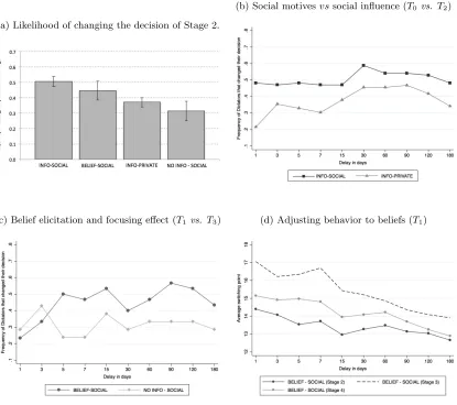
As Panel (a) shows, when Dictators are provided with information about the Recipients’ decisions, changes
in behavior are more likely in the presence of payoff externalities (INFO-SOCIAL: 50.6%vsINFO-PRIVATE:
37.1%) while, in the absence of information, Dictators tend to change their behavior more frequently if beliefs
are elicited (BELIEF-SOCIAL: 44.7% vs NO INFO-SOCIAL: 31.4%).19 Panels (b) and (c) confirm this
19
Table D3 in Appendix D reports the estimated coefficients of a probit regression on the likelihood of changing the decision
Figure 7: Dictators’ decisions in Stage 4
(a) Likelihood of changing the decision of Stage 2.
(b) Social motivesvssocial influence (T0 vs. T2)
(c) Belief elicitation and focusing effect (T1 vs. T3) (d) Adjusting behavior to beliefs (T1)
preliminary evidence disaggregating our observations by time delay. As Panel (b) shows, informed Dictators
are more likely to change their decision when the latter has payoff consequences for the Recipients. Therefore
social motives seem stronger than social influence (p <0.004). On the other hand, Panel (c) shows that, without information, eliciting beliefs seem to trigger social preferences, in that Dictators are more likely to
change their choices in the BELIEF-SOCIAL compared with the NO-INFO-SOCIAL treatment (p <0.096).20
20
When doing pairwise comparisons, we compute, for each Dictator, the frequency of rounds in which the decision was changed
and treat each Dictator as an independent observation. All our findings are robust if we restrict our sample to consistent pairs
Table 4: Choices of Dictators in Stage 4 compared with those of Recipients in Stage 2.
!
T0 T1 T2 T3
INFO-SOCIAL BELIEF-SOCIAL INFO - PRIVATE NO INFO - SOCIAL POOL DATA
(a) Frequency of Recipients’ choices matched by Dictators who moved their choices in Stage 4
Choices move towards the Recipients’ choices 0.67 0.56 0.56 0.29 0.29
Recipients’ choices are perfectly matched 0.15 0.09 0.14 0.06 0.06
Choices move against the Recipients’ choices 0.18 0.36 0.30 0.65 0.65
(b) Tobit regression on the switching point in Stage 4: !!!!= 1−!!!!!+!!!!!!
!
Estimates of alpha 0.262***
0.481***
0.116***
0.050 0.186***
(0.049) (0.146) (0.027) (0.041) (0.028)
Notes. In the Tobit regression, !!"
!
corresponds to the switching point of Dictators in Stage k = {2,4} when the future payment is delayed ! days. The value of !!!
!
denotes the switching of the matched Recipient or the Dictator’s elicited belief. Robust standard errors (clustered at the individual level) in parentheses: ***p<0.01, **p<0.05, *p<0.1!
! !
This latter evidence is in line with the idea of “focusing” put forward by Krupka and Weber [51], where belief
elicitation has a positive effect on pro-social behavior. Finally, Panel (d) shows that Dictators believe that
Recipients are more impatient than they are. Interestingly, Dictators in the BELIEF-SOCIAL treatment
seem to weight their own preferences and beliefs about the Recipients’ preferences and choose a switching
point in Stage 4 that is roughly between the two. This evidence is perfectly in line with our treatment of
social time preferences.
In our paper, we are not only interested in detecting a change of behavior between stages 2 and 4, but
also thedirection of such changes. One question to be addressed is then under which treatment the behavior of the Recipients is better matched by their assigned Dictator. In Panel (a) of Table 4 we disaggregate the
evidence of Figure 7(a) by looking, by treatment, at the relative frequency of Dictators’ choices thati) move
toward,ii) perfectly match oriii) move against the Recipients’ choices (belief) of Stage 2 (3), respectively.
As Table 4 shows, with the exception ofT3, a clear majority of choices in Stage 4 has changed with respect
to Stage 2 in the direction of the Recipients’ preferences.21
Panel (b) of Table 4 provides a quantitative assessment on the statistical significance of such changes by
estimating a double censored tobit model (clustered for subjects) by which the switching point of Dictators
in Stage 4, ϕτ
S4 ∈ {1, ...,21}, is calculated as a convex linear combination between own choices in Stage 2 (ϕτ
S2) and the information received or the Dictator’s elicited beliefs, (ϕτS3):
ϕτ
S4= (1−α)ϕτS2+αϕτS3+ετ.
21
As Panel (b) shows, αis positive and highly significant in all treatments with the exception of T3 (NO
INFO-SOCIAL), this confirming that Dictators’ thresholds move in the direction of those of their groupmates,
once they know (or they reflect upon) the others’ time concerns.22 This effect seems stronger in the presence
of payoff externalities (where social motives apply), but does not vanish without them, as a further sign
of the empirical content of social influence, too. Consistently with our finding in Figure 7, the estimated
α is the highest (lowest) in the BELIEF-SOCIAL (NO INFO-SOCIAL) treatments, respectively. In this
respect, framing the decision of the Dictator as an explicit choice between two selves -whether actual or simply fictitious- seems to work as a necessary condition for a detectable change in behavior in the direction
of the other’s decision. When we look at the intertemporal choices of Stage 4, we indeed find that Dictators
are more likely to follow their own choices of Stage 2 in the PRIVATE compared with the
INFO-SOCIAL (p = 0.019) treatment. Similarly, Dictators are more likely to follow their own choices in the
NO-INFO-SOCIAL compared with the BELIEF-SOCIAL treatment (p <0.037) (see Appendix D3).
4.2
Structural estimations
The estimates of Table 4 show a significant shift in the direction of the Recipient’s decision, conditional upon
i) the provision of some explicit information (or belief) about the latter’s decision, and/orii) a modification of
the incentive structure to experimentally induce payoff externalities. These considerations notwithstanding,
the estimates of Table 4 look at our behavioral evidence on intertemporal decisions only, disregarding the information on individual risk preferences collected in Stage 1. As we already discussed in Section 2, this
may introduce a confound -namely, Dictators’ heterogeneity in own risk concerns- that our own experimental
design can, indeed, control for. This is the reason why we test the robustness of our previous findings by
means of some structural estimations in which we frame (consistent) Dictators’ behavior as maximizing
various parametric random utility functions, some related with the individual decisions of stages 1 to 3,
others which include both the individual (“selfish”) utilities of the Dictator and the Recipient as a result of
some social preference -or social influence- process of joint utility maximization, depending on the treatment.
To this aim, we follow Andersenet al. [4] by conditioning our estimations upon the following stationarity condition:
22
The estimated coefficient for the NO INFO-SOCIAL treatment makes sense only within the realm of some “rational
expectation” hypothesis, since Dictators are never informed about their matched Recipient’s decision. Nevertheless, we report
theT3estimated coefficient for the sake of completeness, and also for a direct comparison with that ofT1, where also Dictators
ui(M0) = ∆i(τ)ui(Mτ), (1)
where ui(x) = x1−ρi/(1−ρi) is a standard (time independent) CRRA utility function and ρi 6= 1 is the risk aversion coefficient. With this parametrization, ρi = 0 identifies risk neutrality, with ρi >0 (ρi <0)
identifying risk aversion (risk loving) behavior, respectively. As in Coller et al. [24], the discount factor is assumed to be ∆i(τ) = βi/(1 +δi)τ, with βi = 1 (βi < 1) in the case of exponential (hyperbolic)
discounting, respectively. The estimations we report in the remainder of this paper follow a standard
“maximum likelihood” approach, by which the estimated parameters (jointly) maximize the likelihood of
observed choices in the different stages of the experiment, conditional on the structural parametrization (1)
and the auxiliary assumption that choices made by the same subject across different stages are statistically
independent.23
In Section 4.2.1 we collect pool estimates of (own) risk (ρ) and intertemporal preferences (β andδ) using
the evidence from Stages 1 to 3. As for social time preferences/influence, Section 4.2.2 estimates the weights
of a social welfare function where individual (own) risk and discounting parameters are estimated separately
for each subject participating to the experiment.
4.2.1 Stages 1-3: individual choices
Table 5 replicates Table 2 in Colleret al. [24] by estimating pool parameters of our structural model (1) using observation from stages 1 to 3. Model 1 imposesβ= 1; i.e., it assumes exponential discounting for all
observations. We remove this assumption in Model 2, which allows for hyperbolic discounting. Finally, we
consider in Model 3 a “binary mixture model” that estimates -jointly with the other behavioral parameters,
ρ,δandβ- the ex-ante probabilities, denoted byπ(1-π), that each individual observation is an independent
draw from Model 2 (Model 1), respectively. The last line of Table 5 replicates our structural estimations
using the evidence from Stage 3 of the BELIEF-SOCIAL treatment.24
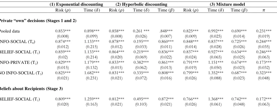
We look first at the pool estimations (first row of Table 5). Our estimates for Model 1 qualitatively confirm
those of Colleret al. [24] in that our (consistent) subjects exhibit significant CRRA and discounting. Similar considerations hold for Model 2: β is significantly smaller than 1, thus providing empirical content to the
23
A detailed description of our identification strategy is presented in Appendix A.
24
As we explained in Section 3, our belief scoring rule is neutral to the (CRRA) risk aversion parametrization, since subjects
either win the price when they guess correctly, otherwise they get nothing. As a consequence, maximizing expected payoffs is
equivalent to maximizing winning probabilities (i.e., our scoring rule only serves the purpose of eliciting the mode of subjects’
belief distribution). Under the assumption that subjects formulate their beliefs using the behavioral model in equation (1) that
Table 5: Risk and time preferences: structural models of individual behavior (Stages 1 to 3).
(1) Exponential discounting (2) Hyperbolic discounting (3) Mixture model
Risk (!) Time (!) Risk (!) Time (!) Time (!) Risk (!) Time (!) Time (!) !
Private “own” decisions (Stages 1 and 2)
Pooled data 0.853*** 0.898*** 0.858*** 0.261 *** .848*** 0.825*** 0.992*** 0.690*** 0.231***
(0.008) (0.099) (0.008) (0.026) (0.007) (0.009) (0.025) (0.014) (0.019)
INFO-SOCIAL (T0) 0.874*** 1.133*** 0.878*** 0.195*** 0.860*** 0.848*** 0.837*** 0.725*** 0.244***
(0.012) (0.215) (0.012) (0.033) (0.011) (0.014) (0.028) (0.026) (0.035)
BELIEF-SOCIAL (T1) 0.859*** 1.133*** 0.864*** 0.219*** 0.836*** 0.837*** 0.927*** 0.634*** 0.246***
(0.02) (0.214) (0.020) (0.069) (0.022) (0.024) (0.065) (0.025) (0.063)
INFO-PRIVATE (T2) 0.829*** 1.179*** 0.833*** 0.382*** 0.861*** 0.791*** 1.151*** 0.674*** 0.173***
(0.015) (0.132) (0.015) (0.062) (0.013) (0.019) (0.050) (0.023) (0.032)
NO INFO-SOCIAL (T3) 0.825*** 1.682*** 0.831*** 0.335*** 0.808*** 0.799*** 1.352*** 0.687*** 0.323***
(0.021) (0.231) (0.021) (0.072) (0.016) (0.026) (0.088) (0.023) (0.048)
Beliefs about Recipients (Stage 3)
BELIEF-SOCIAL (T1) 0.809*** 1.259*** 0.812*** 0.495*** 0.872*** 0.766*** 1.368*** 0.742*** 0.172***
(0.020) (0.163) (0.021) (0.103) (0.021) (0.026) (0.061) (0.048) (0.063)
Notes. Robust standard errors in parentheses *** p<0.01, ** p<0.05, * p<0.1
hyperbolic discounting hypothesis. By the same token, the estimated value of δ significantly drops with
respect to the estimate of Model 1, as it occurs in Coller et al. [24]. When we consider the mixture Model 3, defined as the probability-weighted average of exponential and hyperbolic discounting, we find that the
probability of the latter model being the correct one,π,is estimated to be around 23% and highly significant.
In this sense, we reject the null by which choices can be explained by exponential discounting only.25 The
estimates of the three models disaggregated by treatment suggest little variability across treatments, since we
can never reject the null of joint equality of the estimated coefficients across treatments. Our estimates for
Stage 3 inT1show thatρ(δ) is not as high (low) as the corresponding estimate for Stage 2, which is in line
with the descriptive statistics of Section 4.1: subjects believe that their groupmates are less risk averse and
more impatient (for all models, the corresponding differences are always significant at at least 5 % confidence).
Interestingly enough, our mixture model estimates reveal that subjects’ beliefs underestimate the relevance
of hyperbolic discounting in their groupmates’ decisions, as the estimated value forβis significantly smaller.
We now move to between-subject heterogeneity, which we study by estimating our equation (1) for each
25
We also note that our estimate for π is significantly lower than the one reported by Colleret al. [24] (point estimate:
0.59; std. err. 0.07; 95% confidence interval (0.45,0.74)). This, in turn, seems to be in line with Harrison et al. [6], where
it is suggested that present-bias preferences may be less prominent than previously suggested by the literature. One possible
factor driving our results is that we exclude inconsistent Dictators from the analysis, what may indeed affect our estimates of
consistent subject. Due to lack of observations at the individual level, we can only get estimates for Model
1, where we impose exponential discounting. Let ˆδ = 1+1δ denote the individual discount factor. Figure 8
reports the scatter diagram of the estimated (ˆδ, ρ) pairs characterizing each consistent subject participating
[image:25.612.196.420.240.404.2]to the experiment.
Figure 8: Individual parameter distribution: ˆδvs. ρ
As Figure 8 shows, risk (ρ) and time (ˆδ) preferences are strongly correlated: more risk averse subjects turn out to be also more patient. If we calculate the Spearmann correlation coefficient between ˆδ andρwe get a value of 0.78 (p <0.0001). In this respect, our evidence is consistent with that of Dean and Ortoleva
[27], Burkset al. [18] and Epperet al. [29].
4.2.2 Stage 4: social motivesvs. social influence
Dictators’ choices in Stage 4 are framed as maximizing a welfare function consisting of a convex linear
combination between their own and their assigned Recipient’s risk and intertemporal concerns (precisely,
the individual specific parameters reported in Figure 8):
vk
i(τ) = (1−αi)∆i(τ)
x(τ)1−ρi 1−ρi
+αi∆j(τ)
x(τ)1−ρj 1−ρj
, (2)
whereρj and ∆j(τ) correspond to the risk and discount individual parameters ofi’s assigned Recipient, j.
In this respect, our estimation strategy consists in two steps. We first estimate, the maximum-likelihood
individual estimates for each subject, we estimate the probabilities that any given consistent Dictator i in
Stage 4 resolves the same sequence of intertemporal decisions assuming that i is maximizing the welfare
function (2), derived as the convex linear combination between the utilities of Dictator i and Recipient j,
whether using directlyj’s estimated parameters (treatments INFO-SOCIAL and INFO-PRIVATE), or the
elicited parameters of Stage 3 (treatment BELIEF-SOCIAL).26Table 6 reports our estimation results. Panel
(a) does not condition on whether a consistent Dictator is matched with an in/consistent Recipient. Panel
(b) estimates, separately, two different coefficients,αCP (αCD), depending on whether a consistent Dictator
[image:26.612.132.482.316.472.2]is matched with an (in)consistent Recipient, respectively.
Table 6: Structural model
TR_0 TR_1 TR_2 POOL
INFO-SOCIAL BELIEF-SOCIAL INFO-PRIVATE
(a) Estimates of alpha for consistent Dictators (CD)
alpha (!!"
) 0.739*** 0.612 0.394* 0.527 (0.214) (0.999) (0.204) (0.413)
(b) Estimates of alpha for consistent pairs (CP) of Dictators and Recipients
alpha (!!") 0.758*** 0.612 0.101 0.245 (0.270) (0.999) (0.102) (0.457)
!!:!!
!"
−!!"=0 -0.070 N/A 0.769*** 0.589
(0.292) (0.113) (0.469)
Robust standard errors (clustered at the individual level) in parentheses: *** p<0.01, ** p<0.05, * p<0.1
We look at Model (a) first. Here we see that -somewhat in line with the descriptive statistics of Section
4.1.4- the estimated value of α is positive in all cases. However, it is significant (at 1% confidence) for
treatment T0 (INFO-SOCIAL) and significant only at 10% confidence in the case ofT2 (INFO-PRIVATE).
Things are different when we condition our estimates to the consistency of the REcipient. As panel (b) shows,
the estimate ofαCP in T
0 remains positive and highly significant. The same does not happen inT2, where we cannot reject the null of absence of social influence in our data. The difference between the estimated
αCP in T
0 andT2 is also significant at 5% confidence (p= 0.023), thus suggesting that social motives are
more important than social influence when we only consider pairs composed by consistent Dictators and
Recipients. Along these lines, we find that the effect of being matched with an inconsistent Recipient,αCP
-26
Dictators do not receive any information (nor we elicit their beliefs) in the NO INFO-SOCIAL treatment, therefore equation
αCD, is only significant for T2, which explains why the unconditional estimate of Model (a) is significant.
By contrast, we cannot reject the nullH0 =αCD−αCP = 0 for the INFO-SOCIAL data, which indicates
that behavior of consistent Dictators inT0does not seem to vary significantly depending on the consistency
of the assigned Recipient.
To summarize, once we control for the Dictators’ and Recipients’ estimated risk aversion, both the effects
of the social influence and focusing seem to lose force, compared with our social motives motivating theme.
In particular, the estimated parameter inT1 is never significant, while inT2 is (marginally) significant only
when we do not condition on the consistency of the Recipient.
5
Conclusion
Using evidence from a laboratory experiment, we have tested several complementary working conjectures on
the influence of others in individual intertemporal decisions. According to the “social influence” conjecture,
being simply acknowledged of the choices of someone else is sufficient to trigger a change in behavior;
according to the “focusing” conjecture, forcing subjects to form beliefs over the time preferences of others
is sufficient to move behavior in the direction of beliefs. Our motivating conjecture, instead, calls for social
time preferences as a result of some conscious deliberation in which the others’ intertemporal concerns are
explicitly taken into account when decisions yield payoff externalities.
To different degrees, the descriptive analysis of Section 4.1.4 supports all these working conjectures, as
changes in behavior (in the direction of the Recipient) are more likely in the presence ofi) information about
others’ decisions (even in absence of any payoff externality), ii) belief elicitation (even in absence of any
information about others’ decisions) andiii) payoff externalities (especially in conjunction with information
about others’ decisions). The structural estimations of Section 4.2, however, favor social motives with respect
to the other competing conjectures, especially when we restrict our attention to consistent pairs of Dictators
and Recipients, that is, an environment more in tune with a well defined process of conscious deliberation.
However, it should be noticed that i) this result has been obtained at the cost of a drastic reduction in
the sample size, leaving unexplained the behavior of significant fraction of our subject pool and ii) since
our structural model has been tailored around our social time preference working hypothesis, it is far from
straightforward how to interpret equation (2) within the realm of a model of “social cues” (“focusing”),
in absence of a compelling structural link between the motives (the actions) of Dictators and Recipients,
respectively.
matching processes, where people -when considering intertemporal decisions with payoff externalities- may
cluster or delegate time decisions depending on others’ (risk and) time preferences.
References
[1] Abdellaoui M, L’Haridon O, Paraschiv C (2013).Do Couples Discount Future Consequences Less than
Individuals?, University of Rennes, WP 2013-20.
[2] Ai AC, Norton EC (2003). “Interaction terms in logit and probit models”, Economics Letters, 80(1), 123-129.
[3] Andersen S, Fountain J, Harrison GW, Rutstr¨om EE (2014). “Estimating subjective probabilities”,
Journal of Risk and Uncertainty, 48(3), 207-229.
[4] Andersen S, Harrison GW, Lau M, Rutstr¨om EE (2006). “Elicitation using multiple price lists”, Exper-imental Economics, 9(4), 383-405.
[5] Andersen S, Harrison GW, Lau M, Rutstr¨om EE (2008). “Eliciting Risk and Time Preferences”, Econo-metrica,76(3), 583-618.
[6] Andersen S, Harrison GW, Lau M, Rutstr¨om EE (2014). “Discounting Behavior: A Reconsideration”,
European Economic Review, 71, 15-33.
[7] Anderson JC, Burks SV, DeYoung CV, Rustichini A (2011). Toward the Integration of Personality
Theory and Decision Theory in the Explanation of Economic Behavior, IZA Discussion Paper No.6750.
[8] Andersson O, Holm HJ, Tyran JR, Wengstr¨om E. (2016) “Deciding for Others Reduces Loss Aversion”,
Management Science, 62(1), 29-36.
[9] Andreoni J, Kuhn MA, Sprenger C (2015). “Measuring Time Preferences: A Comparison of
Experi-mental Methods”,Journal of Economic Behavior and Organization, 116, 451-464.
[10] Andreoni J, Sprenger C (2012a). “Estimating Time Preferences from Convex Budgets”,American
Eco-nomic Review, 102(7), 3333-3356.
[11] Andreoni, J, Sprenger C (2012b). “Risk Preferences Are Not Time Preferences”, American Economic
Review, 102(7), 3357-3376.
[13] Banerjee, AV (1992). “A simple model of herd behavior ”, Quarterly Journal of Economics, 107(3), 797-817.
[14] Benhabib J, Bisin A, Schotter A (2010). “Present-bias, quasi-hyperbolic discounting, and fixed costs”,
Games and Economic Behavior, 69(2), 205-223.
[15] Benjamin DJ, Brown SA, Shapiro JM (2013). “Who is ‘behavioral’ ? Cognitive ability and anomalous
preferences”, Journal of the European Economic Association, 11(6), 1231-1255.
[16] Bikhchandani S, Hirshleifer D, Welch I (1992). “A theory of fads, fashion, custom, and cultural change
as informational cascades”, Journal of Political Economy, 100(5), 992-1026.
[17] Browning M (2000). “The Saving Behavior of a Two-Person Household”, Scandinavian Journal of
Economics, 102(2), 235-251.
[18] Burks SV, Carpenter JP, Goette I, Rustichini A (2009). “Cognitive skills affect economic preferences,
strategic behavior, and job attachment”,Proceedings of the National Academy of Sciences, 106, 7745-7750.
[19] Burton RF, Bhagavanlal I, Shivaram B (2009).The Kama Sutra of Vatsyayana, Norilana Books.
[20] Cabrales A, Miniaci R, Piovesan M, Ponti G (2008). “Social Preferences and Strategic Uncertainty: an
Experiment on Markets and Contracts”,American Economic Review, 100(5), 2261-2278.
[21] Chakravarty S, Harrison GW, Haruvy EE, Rutstr¨om EE (2011). “Are You Risk Averse over Other
People’s Money?”,Southern Economic Review, 77(4), 901-913.
[22] Cheung SL (2015). “Comment on ‘Risk preferences are not time preferences: On the elicitation of time
preference under conditions of risk’ ”,American Economic Review, 105 (7), 2242-2260.
[23] Coller M, Williams MB (1999). “Eliciting Individual Discount Rates”, Experimental Economics, 2,
107-127.
[24] Coller M, Harrison GW, Rutstr¨om EE (2012). “Latent Process Heterogeneity in Discounting Behavior”,
Oxford Economic Papers, 64(2), 375-391.
[25] Cubitt R, Starmer C, Sugden R (1998). “On the validity of the random lottery incentive system”,
[26] Cueva C, Iturbe-Ormaetxe I, Mata-Perez E, Ponti G, Sartarelli M, Yu H, Zhukova V (2016).
“Cog-nitive (Ir)Reflection and Behavioral Data: New Experimental Evidence”, Journal of Behavioral and
Experimental Economics, 64, 81-93.
[27] Dean M, Ortoleva P (2012).Is it All Connected? A Testing Ground for Unified Theories of Behavioral Economics Phenomena, Columbia University, mimeo.
[28] Eckel CC, Grossman PJ (2008). “Forecasting risk attitudes: An experimental study using actual and
forecast gamble choices”,Journal of Economic Behavior and Organization, 68, 1-7.
[29] Epper T, Fehr-Duda H, Bruhin A (2011). “Viewing the future through a warped lens: Why uncertainty
generates hyperbolic discounting”,Journal of Risk and Uncertainty, 43(3), 169-203.
[30] Fehr E, Schmidt KM (1999). “A theory of fairness, competition and cooperation”,Quarterly Journal of Economics,114, 817-868.
[31] Feri F, Mel´endez-Jim´enez, MA, Ponti G, Vega-Redondo, F (2011). “Error cascades in observational
learning: An experiment on the chinos game”,Games and Economic Behavior, 73(1), 136-146.
[32] Fischbacher U (2007). “z-Tree: Zurich toolbox for ready-made economic experiments”, Experimental
Economics, 10(2), 171-178.
[33] Frederick S (2005). “Cognitive reflection and decision making”, Journal of Economic Perspectives,19, 24-42.
[34] Frederick S, Loewenstein G, O’Donoghue T (2002). “Time Discounting and Time Preference: A Critical
Review”,Journal of Economic Literature, 40, 351-401.
[35] Frignani N, Ponti G (2012). “Social vs. Risk Preferences under the Veil of Ignorance”,Economics Letters, 116, 143-146.
[36] Glaeser E, Laibson D, Scheinkman J, Soutter C (2000). “Measuring trust”,Quarterly Journal of Eco-nomics,115, 811-846.
[37] Goeree JK, Yariv L (2015). “Conformity in the Lab”, Journal of the Economic Science Association, 1-14.
[39] Harrison GW, Lau M, Rutstr¨om EE (2013). “Identifying Time Preferences with Experiments:
Com-ment.”, Center for the Economic Analysis of Risk Working Paper WP-2013-09.
[40] Harrison GW, Lau M, Rutstr¨om EE, Sullivan MB (2005). “Eliciting Risk and Time Preferences Using
Field Experiments: Some Methodological Issues”, in J. Carpenter, G.W. Harrison and J.A. List (eds.),
Field Experiments in Economics, Greenwich, CT, JAI Press, Research in Experimental Economics, Volume 10, Emerald Group Publiushing Limited, 41-196.
[41] Harrison GW, Lau M, Rutstr¨om EE, Tarazona-Gomes M (2013). “Preferences over social risk”,Oxford Economic Papers, 65, 25-46.
[42] Harrison GW, Miniaci R, Ponti G.Social Preferences over Utilities, LUISS Guido Carli, mimeo.
[43] Harrison GW, Rutstr¨om EE (2008). “Risk Aversion in the Laboratory”, in Cox JC, Harrison GW
(eds.), Risk Aversion in Experiments (Research in Experimental Economics, Volume 12), Emerald
Group Publishing Limited, 41-196.
[44] Hey JD, Lee J (2005). “Do Subjects Separate (or Are They Sophisticated)?”,Experimental Economics, 8, 233-265.
[45] Hey JD, Orme C (1994). “Investigating Generalizations of Expected Utility Theory Using Experimental
Data”,Econometrica, 62(6),1291-1326.
[46] Holt CA, Laury SK (2002). “Risk Aversion and Incentive Effects”,American Economic Review,92(3), 1644-1655.
[47] Holt CA, Laury SK (2005). “Risk Aversion and Incentive Effects: New Data without Order Effects”,
American Economic Review,95(3), 902-904.
[48] Hung AA, Plott CR (2001). “Information cascades: Replication and an extension to majority rule and
conformity-rewarding institutions”, American Economic Review, 91(5), 1508-1520.
[49] Karaca-Mandic P, Norton EC, Dowd B (2012). “Interaction terms in nonlinear models”,Health services research, 47(1), 255-274.
[50] Kovarik J (2009). “Giving it now or later: Altruism and discounting”,Economics Letters, 102(3), 152-154.
[52] Laury SK, McInnes MM, Swarthout JT (2012). “Avoiding the curves: Direct elicitation of time
prefer-ences”,Journal of Risk and Uncertainty, 44, 181-217.
[53] Lazaro A, Barberan R, Rubio, E (2001). “Private and social time preferences for health and money: An
empirical estimation”,Health Econo