Short Term Forecasting Analysis for Municipal Water Demand

Munich Personal RePEc Archive

Short-Term Forecasting Analysis for

Municipal Water Demand

Fullerton, Thomas M., Jr. and Ceballos, Alejandro and

Walke, Adam G.

University of Texas at El Paso

26 June 2015

Online at

https://mpra.ub.uni-muenchen.de/78259/

Short-Term Forecasting Analysis for Municipal Water Demand*

1

Department of Economics & Finance, University of Texas at El Paso, El Paso, TX 79968-0543, Telephone 915-747-7747, Facsimile 915-747-6282, Email tomf@utep.edu

* A revised version of this study appears in Journal of the American Water Works Association, 108 (1), E27-E38, doi: 10.5942/jawwa.2016.108.0003

Abstract

Short-term water demand forecasts inform decisions regarding budgeting, rate design, water supply system operations, and effective implementation of conservation policies. This study develops a Linear Transfer Function (LTF) forecasting model for El Paso, Texas, a growing city located in the desert Southwest region of the United States. The model is used to generate monthly-frequency out-of-sample simulations of water demand for periods when actual demand is known. To measure the accuracy of the LTF projections against viable alternatives, a set of benchmark forecasts is also developed. Both descriptive accuracy metrics and formal statistical tests are used to analyze predictive performance. The LTF model outperforms the alternatives in predicting demand per customer but falls a little short in projecting growth in the customer base. Changes in climatic and economic conditions are found to impact consumption per customer more rapidly than changes in water rates.

Keywords

Water demand models, water conservation, forecast accuracy

Acknowledgements

The Water Research Foundation provided financial, technical, and administrative support for the research upon which this manuscript is based. Additional financial support was provided by El Paso Water Utilities, Hunt Communities, City of El Paso Office of Management & Budget, and the University of Texas at El Paso. Helpful comments and suggestions were provided by David Torres, Marcela Navarrete, Jack Kiefer, Chris Meenan, Paul Merchant, Michael McGuire, Andrew Eaton, and two anonymous referees. Econometric research assistance was provided by Juan Cárdenas.

INTRODUCTION

simulations of future water consumption dynamics can aid policymakers in targeting conservation measures for optimal effectiveness (Memon & Butler, 2006).

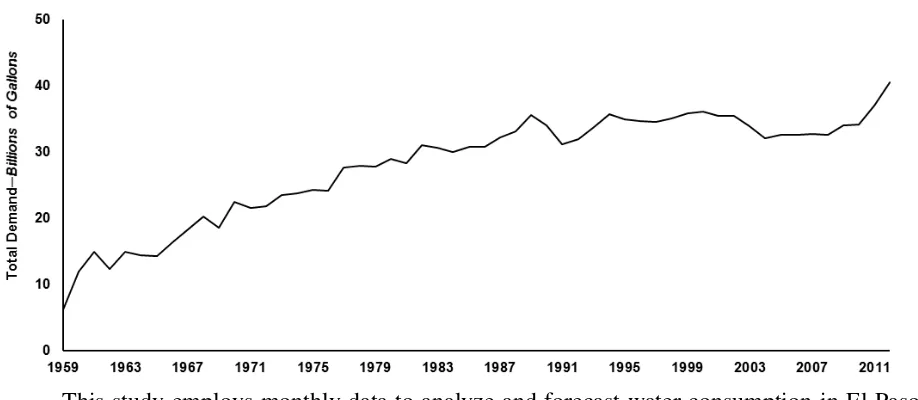
The objective of this study is to analyze short-term water consumption dynamics in El Paso, Texas. A growing metropolitan economy located in the desert Southwest region of the United States, El Paso has historically faced pronounced water supply constraints. Recurring droughts place additional pressure on local water supplies (Washington-Valdez, 2013). In response to projected shortages, El Paso Water Utilities (EPWU) adopted a comprehensive conservation strategy in 1991 (Tennyson & Parker, 2007). The subsequent moderation in the annual growth of water consumption is shown in Figure 1. Water demand forecasts and simulations are useful for both designing and evaluating conservation policies such as those put in place by EPWU in recent decades (Little & Moreau, 1991; White et al., 2003). Also, an arid climate, a growing population, and scarce water resources combine to make reliable forecasts essential to ensuring an adequate supply of water during peak-demand seasons in El Paso.

Figure 1. Total water consumption in El Paso, 1959-2012

This study employs monthly data to analyze and forecast water consumption in El Paso. A similar study was conducted for this region by developing a Linear Transfer Function (LTF) model with monthly data from 1994 to 2002 (Fullerton & Elias, 2004). This effort expands the original sample size by 11 years. The larger sample includes more business cycles, which may shed some light on how municipal water usage responds to fluctuations in economic conditions. The next section reviews the literature on water demand modeling and forecasting. Section three includes a discussion of the data and the methodological framework employed. Empirical results are then presented, followed by a conclusion and policy implications.

LITERATURE REVIEW

water-saving lawn irrigation technology, and introducing xeriscaping enhances the capacity of consumers to respond to price hikes by reducing water usage in the long-run.

A long-running debate regarding the choice between average and marginal price measures is well documented. Several studies concerned with estimating demand equations for water and electricity report that consumers react to average price (Ito, 2014; Nieswiadomy, 1992; Shin, 1985; Foster & Beattie, 1981). Failure to understand block pricing structures, the small portion of income that the total bill represents, and high information costs are all possible explanations of consumer propensities for utilizing ex post average prices as proxies for marginal prices. Other studies provide evidence in favor of marginal prices and suggest that endogeneity bias arises when average prices are employed (Williams & Suh, 1986; Williams, 1985).

Market and non-market conservation efforts are useful tools for managing water demand. Market conservation efforts consist of increasing price to achieve lower consumption levels. Price elasticities are not uniform across all income levels; there is evidence that low income households exhibit elasticities up to five times higher than their wealthier counterparts (Agthe & Billings, 1987; Renwick & Archibald, 1998). It follows that price conservation efforts disproportionately affect consumption in lower income households. Non-market conservation programs such as public awareness initiatives, education campaigns, and provision of additional information on marginal rates effectively increase price responsiveness, thereby achieving desired conservation levels with smaller price increases (Michelsen et al., 1999; Moncur, 1987).

Fullerton and Elias (2004) estimate short-term water demand forecasts in El Paso as a function of economic and climatic variables. Monthly forecasts are generated employing a LTF methodology and are then compared to a random walk benchmark. The study concludes that the LTF outperforms the benchmark at every forecast step-length. Two subsequent studies conducted for Ciudad Juarez and Tijuana confirm these results (Fullerton et al., 2007; Fullerton et al., 2006). The study at hand conducts a similar exercise using a larger sample that includes various episodes of economic downturns and recoveries. In addition, a broader spectrum of forecast accuracy evaluation metrics will be employed as described in the next section.

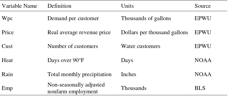
DATA AND METHODOLOGY

Total water demand for El Paso is decomposed into per customer demand (Wpc) and the total number of customers (Cust), with each component modeled separately (Fullerton & Schauer, 2001). Per customer water consumption is obtained by dividing total water billed by the number of customers and is then modeled as a function of average price (Price), days with peak temperatures above 90°F (Heat), total precipitation (Rain), and nonfarm employment (Emp). Because price figures are not always available, other studies have circumvented this obstacle by dividing revenue over consumption to approximate average price (Shin, 1985). This paper follows the same procedure. While providing only an approximation of relevant rates, this approach has been shown to yield econometric results in line with other price measures (Dalhuisen et al., 2003; Nieswiadomy & Molina, 1991). The average price figures are deflated using the consumer price index (CPI) to obtain real values in 1982-1984 dollars.

inches are retrieved from the National Oceanic and Atmospheric Administration. Non-seasonally-adjusted nonfarm employment and CPI are collected from the Bureau of Labor Statistics. Due to the unavailability of monthly personal income series at the regional level, employment is used as a proxy for economic conditions. Table 1 defines each variable and lists data sources.

Table 1. Variables used for water demand and customer base modeling

Variable Name Definition Units Source

Wpc Demand per customer Thousands of gallons EPWU

Price Real average revenue price Dollars per thousand gallons EPWU

Cust Number of customers Water customers EPWU

Heat Days over 90°F Days NOAA

Rain Total monthly precipitation Inches NOAA

Emp Non-seasonally adjusted

nonfarm employment Thousands BLS

The LTF ARIMA (autoregressive integrated moving average) methodology is used to model demand. This methodology is an extension of the process outlined by Box and Jenkins (1976). Previous efforts have utilized LTF ARIMA for forecasting demand for water and natural gas (Fullerton & Elias, 2004; Fullerton & Nava, 2003; Liu & Lin, 1991). Differencing is applied to each data series to achieve the required stationarity condition. The cross-correlation functions between stationary components of the dependent and independent variables are plotted and inspected to determine potential lag structures of the explanatory variables. Autoregressive (AR) and moving average (MA) components are subsequently introduced into the model to account for any systematic variation in the dependent variable not explained by the preliminary multiple input transfer function (Wei, 2006). Potential ARMA (autoregressive and/or moving average) parameters are identified by looking for significant autocorrelation and partial autocorrelation coefficients in the correlogram of the residuals. The specification of the LTF is shown in Equation (1); the hypothesized coefficient signs are included parenthetically.

𝐷𝑝𝑐𝑡= 𝛼0+ ∑ 𝛽𝑎 𝐴

𝑎=1

𝐴𝑝𝑡−𝑎+ ∑ 𝛽𝑏𝐻𝑒𝑎𝑡𝑡−𝑏 𝐵

𝑏=1

+ ∑ 𝛽𝑐𝑅𝑎𝑖𝑛𝑡−𝑐 𝐶

𝑐=1

+ ∑ 𝛽𝑑𝐸𝑚𝑝𝑡−𝑑 𝐷

𝑑=1

+ ∑ 𝜙𝑖𝐷𝑝𝑐𝑡−𝑖 𝑝

𝑖=1

+ ∑ θ𝑗𝑢𝑡−𝑗 𝑞

𝑗=1

+ 𝑢𝑡

(-) (+) (-) (+) (1)

water demand are expected to be positively correlated with prevailing regional economic conditions. Therefore the parameters for employment should be positive.

As mentioned above, average price is calculated by dividing total revenue by water consumption. Because the latter is also the dependent variable in Equation (1), it is necessary to test for endogeneity (Fullerton et al., 2013). This is accomplished using an artificial regression test (Davidson & MacKinnon, 1989). Two instrumental variables are used to conduct the test. The capital stock deflator for water supply facilities is obtained from the Bureau of Economic Analysis. Another instrument, a unit labor cost index for water utilities, is retrieved from the Bureau of Labor Statistics. Both instruments are adjusted for inflation using the CPI. The artificial regression procedure is used to evaluate the null hypothesis that average price is uncorrelated with the error term in Equation (1).

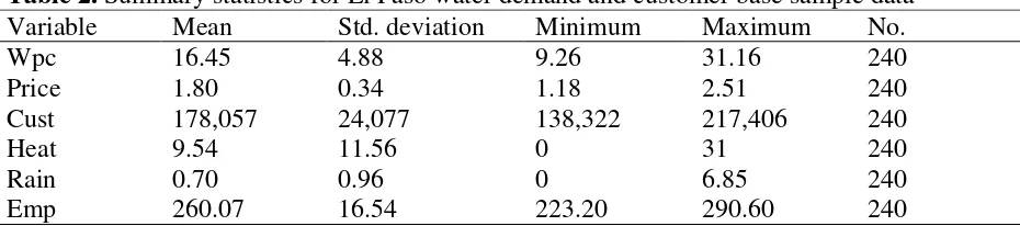
To estimate total water demand, it is necessary to model the number of customers in addition to per customer demand. Multiple studies have estimated the customer base for water utilities in metropolitan areas as functions of economic variables (Fullerton et al., 2007; Fullerton et al., 2006). Following a similar approach, this study constructs a single input transfer function where nonfarm employment and ARMA terms are used as regressors (Equation 2). Employment is expected to be positively correlated with the size of the customer base. The equation and the hypothesized sign are expressed below, followed by summary statistics for the sample data in Table 2.

𝐶𝑢𝑠𝑡𝑡 = 𝛼0+∑𝑎=1𝐴 𝛽𝑎𝐸𝑚𝑝𝑡−𝑎+∑𝑝𝑖=1𝜙𝑖𝐶𝑢𝑠𝑡𝑡−𝑖+ ∑𝑞𝑗=1θ𝑗𝑣𝑡−𝑗+ 𝑣𝑡 (2) (+)

Table 2. Summary statistics for El Paso water demand and customer base sample data

Variable Mean Std. deviation Minimum Maximum No.

Wpc 16.45 4.88 9.26 31.16 240

Price 1.80 0.34 1.18 2.51 240

Cust 178,057 24,077 138,322 217,406 240

Heat 9.54 11.56 0 31 240

Rain 0.70 0.96 0 6.85 240

Emp 260.07 16.54 223.20 290.60 240

Development of a vector autoregression (VAR) model provides a benchmark that allows for forecast accuracy comparisons with respect to the LTF ARIMA model. Although VAR models are more commonly employed for macroeconomic simulations, some studies have utilized them for modeling and forecasting regional economies (Cargill & Morus, 1988; Kinal & Ratner, 1986). A basic VAR model of order p can be written as shown in Equation (3).

𝑦𝑡= 𝐴0+ 𝐴1𝑦𝑡−1+ ⋯ + 𝐴𝑝𝑦𝑡−𝑝+ 𝑢𝑡 (3)

Where yt is a vector containing k time series variables, A0 is a vector of constant terms, the Ai’s for i= 1,…,p are k × k coefficient matrices, and ut is a vector of random disturbances (Lütkepohl & Krätzig, 2004). Only predetermined variables are included on the right-hand-side of (3) and the error terms are assumed to be serially uncorrelated and homoscedastic. If the assumptions are satisfied, ordinary least squares estimates of the VAR parameters are consistent and asymptotically efficient (Enders, 2010).

Hannan-Quinn information criteria (Clarke & Mirza, 2006). Optimal lag structures are those associated with the minimum values of these criteria. The basic model shown in Equation (3) can be augmented by including exogenous stochastic variables as regressors in each of the k

equations. In the case that exogenous variables are added to the list of regressors, explanatory equations are not included for those variables as part of the system (Lütkepohl & Krätzig, 2004). Examples of exogenous variables that might be incorporated into a VAR model of economic conditions include weather indicators and dummy variables to account for calendar effects (Hendry & Nielsen, 2007).

There is some controversy surrounding whether the data used to estimate a VAR need to be stationary (Enders, 2010). To obtain parameter estimates that appropriately describe the relationships between variables, Ashley and Verbrugge (2009) recommend differencing any non-stationary data prior to estimating the VAR unless the variables are cointegrated. Because the variables in the sample are non-stationary in level form, cointegration testing is conducted. If the variables are found to be cointegrated, the VAR will be estimated using data in level form; otherwise, the data will be differenced to achieve stationarity. Finally, a VAR Lagrange Multiplier (LM) test is carried out on the residuals to test for serial correlation at the selected lag order.

Once the LTF ARIMA and VAR models are developed, each is used to generate ex-post

forecasts of water demand. Random Walk (RW) and Random Walk with Drift (RWD) benchmark forecasts are also calculated. For the customer base, the RW forecast is equal to the number of customers in the month before the start of the forecast period. For demand per customer, the RW projection is equal to the level of consumption recorded in the same month of the previous year. The RWD forecast is equal to the RW forecast plus the average monthly change over the course of a year. To evaluate the four sets of projections, several measures of forecast accuracy are employed: the Theil inequality coefficient, an error differential regression test, and a non-parametric test for directional accuracy.

The Theil inequality coefficient, also called a U-statistic, is based on the root-mean squared error and provides a descriptive measure of forecast accuracy with values ranging from zero to one (Theil, 1961). A value of zero indicates the best possible fit is attained; the converse is true when the statistic equals one. The second moment of the U-statistic can be further decomposed into three proportions of inequality to extract additional information about forecast accuracy: bias (UM), variance (US), and covariance (UC). The bias proportion provides a measure of systematic divergence between the means of actual and predicted demand. The variance proportion reflects the forecast’s ability to replicate variation in water consumption. The covariance proportion represents unsystematic error. The sum of the three proportions is equal to one with an ideal distribution of 𝑈𝑀 = 𝑈𝑆 = 0 and 𝑈𝐶 = 1 (Pindyck & Rubinfield, 1998).

An error differential regression test is used to determine whether the difference between the errors from two competing forecasts is statistically significant (Ashley et al., 1980). The procedure consists of testing the null hypothesis shown in Equation (4).

H0: MSE(𝑒1) − MSE(𝑒2) = 0 (4)

MSÊ(𝑒1) − MSÊ(𝑒2) = [cov̂ (Δ, Σ)] + [m(𝑒1)2− m(𝑒2)2] (5)

Where cov̂ is the sample covariance and m denotes sample mean. Assuming the means of both sets of errors have the same sign, a test of cov(Δ,Σ) = μ(Δ) = 0 can be used to evaluate the null hypothesis. Equation (6) provides a specification suitable for testing that hypothesis. When the error means have opposite signs, Equation (7) is utilized instead.

Δ𝑡= 𝛽1+ 𝛽2[Σ𝑡− 𝑚(Σ𝑡)] + 𝑢𝑡 (6)

Σ𝑡 = 𝛽1 + 𝛽2[Δ𝑡− 𝑚(Δ𝑡)] + 𝑢𝑡 (7)

In Equations (6) and (7), ut is a randomly distributed error term. A positive value for

𝛽2indicates that the second forecast outperforms the first one. The interpretation of β1 depends

on the sign of e1’s mean. If β1 has the same sign as e1, the second forecast is judged superior. Guidelines on determining whether or not to reject the null hypothesis based on t- and F -statistics are given in Ashley et al. (1980).

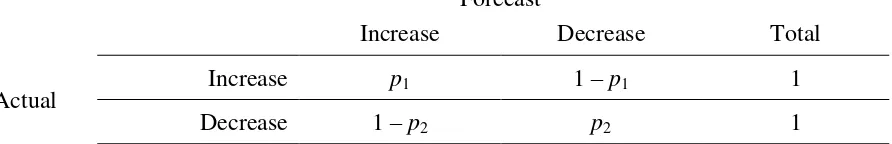
Directional forecast evaluations assess the ability of a model to correctly predict the direction of change in the variable of interest. A contingency table, like Table 3, is usually employed in these procedures to compare the forecasted increases and decreases in demand to the actual directions of change. The probability values p1 and p2 reflect the proportion of correct predictions of directional change while the off-diagonal probabilities reflect the proportion of incorrect predictions.

Table 3. Probability value contingency table

Forecast

Increase Decrease Total

Actual

Increase p1 1 – p1 1

Decrease 1 – p2 p2 1

The table is based on directions of movement in the dependent variable relative to the prior observation and whether the current value is higher or lower than that of the previous period.

Henriksson and Merton (1981) propose a test of the null hypothesis that a set of forecasts provides no useful information regarding the direction of change in a given variable. This hypothesis can be stated in terms of the probabilities shown in Table 3 as H0: p1+p2= 1. For a model that always predicts the correct direction of change, p1 and p2 will each be equal to one and p1+p2= 2. Conversely, a model that always generates the wrong predictions will have values of zero for both of those probabilities and the probability values for the off-diagonal elements will sum to two. Under the null hypothesis the forecasts of directional change are independent of the actually observed directional changes.

changes in the opposite direction of the changes that are actually observed. Therefore, a one tailed test is recommended for the modified null hypothesis: p1+p2 ≤ 1. Cumby and Modest (1987) point out that the null hypothesis can be evaluated using a Fisher exact test.

EMPIRICAL RESULTS

Table 4 shows LTF ARIMA estimation results for the per customer water demand equation. The series are seasonally and first differenced prior to estimation to induce stationarity. All of the independent variables affect demand within three months. The estimated coefficients associated with every explanatory variable are significant at the 95% confidence level and the coefficient signs are as hypothesized. One AR and two MA parameters are included to correct for residual serial correlation (a statistical glossary is included in Table 8).

Movements in the real average price negatively affect water demand with a lag of three months. A number of other studies also find evidence that consumers respond to lagged, rather than contemporaneous, values of average price (Fullerton et al., 2007; Arbues & Villanua, 2006; Arbues et al., 2004; Fullerton & Nava, 2003). This is consistent with the argument that customers base consumption decisions on price information acquired from bills for water that has already been consumed in prior periods (Charney & Woodard, 1984). The elasticity estimate calculated by multiplying the own-price coefficient from Table 4 by the ratio of mean price to mean demand is -0.32. This is somewhat smaller in magnitude than the average price elasticity estimate of -0.41 reported by Dalhuisen et al. (2003) in a meta-analysis of previous water demand studies.

Because total water consumption is used to calculate both average price and the dependent variable, it is possible that the price variable may be endogenous. However, the results of an artificial regression test indicate the absence of feedback between water demand and contemporaneous values of average price (Davidson & MacKinnon, 1989). Some previous studies also report that average water price variables are exogenous (Mylopoulos et al., 2004; Nauges & Thomas, 2000; Nieswiadomy, 1992). Repeating the artificial regression test for lagged values of average price yields conflicting results. However, lagged values of the average price variable are predetermined and are treated as exogenous for the purposes of this study. This is in line with research on electricity demand that uses lagged average price as an instrumental variable for contemporaneous average price on the grounds that the lagged values are exogenous (Aroonruengsawat et al., 2012).

The number of days when the temperature exceeds 90° Fahrenheit and its first order lag indicate higher temperatures exert a positive impact on water usage. Conversely, precipitation is associated with lower consumption levels after a one month lag. The effects of weather conditions on per customer water consumption are similar to those reported for the same region in Fullerton and Elias (2004). The number of days with rain and monthly maximum temperature are not found to exert statistically significant impacts on demand and aretherefore excluded from the model.

employment levels on per customer water consumption in El Paso is consistent with the results of previous studies for this region and others (Musolesi & Nosvelli, 2011; Fullerton & Elias, 2004).

Table 4. LTF ARIMA – El Paso water demand per customer model results Dependent Variable: Wpc

Sample (adjusted): May 1996 – December 2013

Variable Coefficient Standard error t-Statistic Probability

C 0.001451 0.003646 0.397972 0.6911

Price(-3) -2.898840 0.778962 -3.721412 0.0003

Heat 0.088971 0.017208 5.170437 0.0000

Heat(-1) 0.130562 0.018816 6.939010 0.0000

Rain(-1) -0.395477 0.071969 -5.495121 0.0000

Emp 0.120658 0.038938 3.098746 0.0022

AR(12) -0.295368 0.068062 -4.339688 0.0000

MA(1) -0.705800 0.044613 -15.82044 0.0000

MA(12) -0.265299 0.047262 -5.613349 0.0000

R-squared 0.702113 Mean dependent variable 0.003356

Adjusted R-squared 0.690373 S.D. dependent variable 1.611280

S.E. of regression 0.896582 Akaike info criterion 2.661072

Sum of squared residuals 163.1836 Schwarz criterion 2.803569

Log likelihood -273.0737 Hannan-Quinn criterion 2.718666

F-statistic 59.80824 Durbin-Watson statistic 1.962049

Probability (F-statistic) 0.000000

structure is also shown in Table 4. Those changes may also result as a consequence of using a larger data set that potentially allows for more accurate statistical inference. Although wholesale changes to this model specification do not occur, failure to regularly update parameter estimates as new data become available will tend to increase the risk of predictive inaccuracy.

Another observation on model characteristics can be made with respect to Table 4. The data for this study are for municipal water consumption in El Paso, a fairly unique metropolitan economy located in a semi-arid geographical region. The basic framework is applicable to other metropolitan economies that may receive higher volumes of precipitation and observe lower annual average temperatures (Fullerton et al., 2013). Even though the model specifications for other regions may be similar to that shown in Table 4, the parameter magnitudes can differ substantially. For example, residential water consumption in a rainy environment is likely to be less responsive to precipitation than is the case in El Paso. A coefficient estimate for such a data sample would likely be smaller, in absolute magnitude, than what is reported in Table 4. Similarly, temperature variations may not cause consumption to react as much in regions where the climate is more moderate than it is in the desert southwest of the United States.

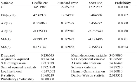
Table 5. LTF ARIMA – El Paso customer base model results Dependent Variable: Cust

Sample (adjusted): May 1996 – December 2013

Variable Coefficient Standard error t-Statistic Probability

C 345.1983 22.65783 15.23527 0.0000

Emp (-32) 42.43972 12.24930 3.464666 0.0007

AR(12) 0.368860 0.067597 5.456777 0.0000

AR(18) -0.175113 0.062910 -2.783540 0.0060

MA(1) -0.299312 0.072622 -4.121496 0.0001

MA(3) 0.157147 0.072865 2.156673 0.0324

R-squared 0.236645 Mean dependent variable 346.9096

Adjusted R-squared 0.214324 S.D. dependent variable 319.6505

S.E. of regression 283.3329 Akaike info criterion 14.16443

Sum of squared residuals 13727458 Schwarz criterion 14.27210

Log likelihood -1247.552 Hannan-Quinn criterion 14.20810

F-statistic 10.60219 Durbin-Watson statistic 2.013352

Probability (F-statistic) 0.000000

sign and statistical significance of the constant term denotes a very steady rate of growth in the customer base. Nonfarm employment enters the equation with a lag of 32 months. The 32 period lag suggests it takes almost three years for the customer base to respond to movements in employment. Previous research on border region water demand also reports that the response to business cycle fluctuations occurs after relatively long delays. Studies conducted for Tijuana and Ciudad Juarez find that the customer base reacts to changes in maquiladora employment levels after lags of up to 16 and 18 months, respectively (Fullerton et al., 2007; Fullerton et al., 2006). ARMA parameters are introduced to correct for serial correlation.

This paper follows the approach of a previous study that employed a Bayesian VAR model as a benchmark for structural forecasts in the El Paso-Juarez border region (Fullerton, 2001). VARs provide a natural alternative to transfer functions since they require imposing fewer exclusion restrictions (Enders, 2010; Sims, 1980). Two VAR models are developed as benchmarks to allow for forecast accuracy comparisons with respect to the LTF models. The first model estimates water demand per customer and real average price. The second model includes the number of customers and nonfarm employment.

As described in the previous section, non-stationary time series must be differenced prior to estimating a VAR unless those series are cointegrated. A Johansen cointegration test conducted for the residuals in the demand-price VAR yields conflicting results (Johansen, 1991). The trace rank test indicates the equations are cointegrated, whereas the maximum eigenvalue rank test suggests there are no cointegrated series. Further testing is required to determine whether the series are cointegrated. An Engle-Granger two-step procedure finds no evidence of cointegration at the 95% confidence level (Engle & Granger, 1987). As a result, the series are first and seasonally differencedto achieve stationarity. A lag order of12 is selected based on the Akaike information criterion. One- and two-month lags of three exogenous variables are also included in the VAR. The exogenous variables aremonthly precipitation, employment, and days with temperatures exceeding 90°F. The results from a VAR residual LM test suggest serial correlation is not problematic (Johansen, 1995).

Impulse response functions trace how each endogenous variable responds over time to a shock in a particular variable (Pindyck & Rubinfield, 1998). The impulse response function for demand and average price is presented in Figure 2, where a change of one standard deviation is applied to the residual of average price at period t. A shock in average price has a strong negative effect on demand after four months and subsequent reactions oscillate around zero.

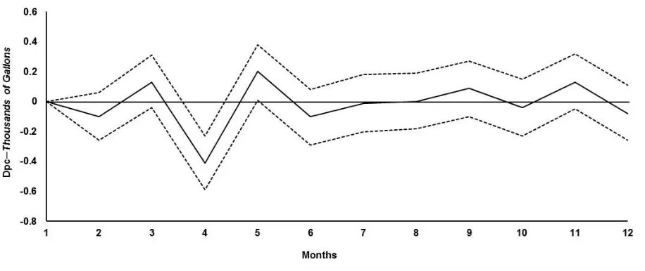
The second VAR is estimated with customers and nonfarm employment as the endogenous variables. Both components of the Johansen cointegration test indicate there is no evidence of cointegration at the 95% confidence level. Employment requires seasonal and first differencing; the customer base requires only first differencing. Similarly to the first VAR, the Akaike information criterion favors a 12 order lag specification. The exogenous variables are not found to exert statistically reliable impacts on either of the endogenous variables and inclusion of exogenous variables results in higher values of the information criteria for the overall system. Because of this, the model is re-estimated using only the two endogenous variables. The impulse response function for customers and employment is provided in Figure 3. The external shock in employment does not generate a pronounced effect on the customer base within twelve months; the response fluctuates around zero and disappears after 5 periods.

Figure 3. Response of Cust to a one standard deviation innovation in Emp ± 2 standard error

OUT-OF-SAMPLE SIMULATION RESULTS

Theil Inequality Coefficients for per customer demand forecasts indicate that the LTF model outperforms the alternatives across all forecast periods. Furthermore, the second moment decompositions of the U-statistics suggest that the LTF model successfully replicates systematic movements in water usage. For the VAR demand forecasts, the distribution of the proportions of inequality rapidly deviates from the optimal distribution as the step lengths increase. These results are in line with a previous study where VAR models were found to generate less accurate forecasts than structural macroeconomic models for several variables of interest (Bischoff et al., 2000).

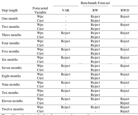
Table 6. Error differential regression test results for El Paso water usage and customer base forecasts

Benchmark Forecast

Step length Forecasted

Variable VAR RW RWD

One month Wpc - Reject Reject

Cust - Reject -

Two months Wpc - Reject Reject

Cust - Reject -

Three months Wpc Reject Reject Reject

Cust - Reject -

Four months Wpc Reject Reject Reject

Cust - Reject -

Five months Wpc Reject Reject Reject

Cust - Reject -

Six months Wpc Reject Reject Reject

Cust - Reject -

Seven months Wpc Reject Reject Reject

Cust - Reject -

Eight months Wpc Reject Reject Reject

Cust - Reject -

Nine months Wpc Reject Reject Reject

Cust - Reject -

Ten months Wpc Reject Reject Reject

Cust - Reject -

Eleven months Wpc Reject Reject Reject

Cust - - Reject

Twelve months Wpc Reject Reject Reject

Cust - - Reject

The null hypothesis tested is that of mean squared error equality.

Rejection of the null hypothesis indicates that the LTF equation forecasts are most accurate.

more accurate for five step lengths each. The LTF, VAR, and RWD forecasts are very close to one another in terms of accuracy for the twelve step lengths. The bias proportion increases rapidly for the LTF and VAR forecast errors as the horizon increases and, after six months, it accounts for more than half of the out-of-sample errors. The RWD forecast errors do not exhibit such a rapid increase in the proportion of bias, but the variance proportion increases faster than in the rest of the forecasts.

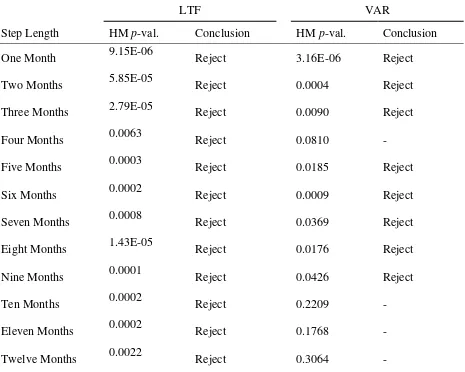
Table 7. Directional accuracy tests for El Paso water demand per customerforecasts

LTF VAR

Step Length HM p-val. Conclusion HM p-val. Conclusion

One Month 9.15E-06 Reject 3.16E-06 Reject

Two Months 5.85E-05 Reject 0.0004 Reject

Three Months 2.79E-05 Reject 0.0090 Reject

Four Months 0.0063 Reject 0.0810 -

Five Months 0.0003 Reject 0.0185 Reject

Six Months 0.0002 Reject 0.0009 Reject

Seven Months 0.0008 Reject 0.0369 Reject

Eight Months 1.43E-05 Reject 0.0176 Reject

Nine Months 0.0001 Reject 0.0426 Reject

Ten Months 0.0002 Reject 0.2209 -

Eleven Months 0.0002 Reject 0.1768 -

Twelve Months 0.0022 Reject 0.3064 -

The null hypothesis is that the forecasts fail to predict directional changes in demand.

Rejection of the null hypothesis indicates that the forecasts provide useful information regarding directional changes in demand.

results for demand and customers are shown in Table 6. In the case of per customer demand, the LTF outperforms the VAR by a statistically significant margin for ten forecast step-lengths and improves on the accuracy of the random walks in every period. By contrast, the errors from the VAR and LTF forecasts of the customer base are nearly identical in size and thus the hypothesis of equality cannot be rejected at any step-length. The LTF represents a significant improvement over the RW for the first 10 step lengths but it only outperforms the RWD projections by a statistically significant margin for the last two step lengths.

Directional forecast evaluations determine a model’s ability to accurately predict the direction of change in a variable of interest. These tests are only conducted for water demand because the customer base increases in nearly every period throughout the forecast sample. The null hypothesis states that the forecast fails to predict directional changes in demand per customer (Henriksson & Merton, 1981). Consequently, rejection of the null implies the model successfully predicts the direction of the movements in water usage. The results for the LTF and VAR forecasts are summarized in Table 7. The null is rejected at every step length for the LTF and for eight of twelve step-lengths in the case of the VAR. This indicates that the LTF is more suitable for out of sample simulations than the VAR.

CONCLUSION

This study applies various methodologies to estimate models of water demand in El Paso, Texas, and compares the short-run forecasting accuracy of each model. The LTF ARIMA parameter estimates indicate that a 10 % rate increase will lead to a 3.2 % decline in water demand after a lag of three months. Impulse response functions generated using the VAR model also suggests that prices negatively impact demand after a multi-month lag. These outcomes imply that price increases can serve as an instrument for controlling the growth of water consumption in El Paso. However, the results also indicate that the full effect of rate changes may not be felt immediately as price information is typically gleaned from bills for water already consumed. Furthermore, consumers in El Paso appear to react rather quickly, within one month, to changing weather conditions. Thus, in the event of a severe drought, it is likely that non-price conservation measures such as public information campaigns will be needed in addition to appropriate price signals in order to rapidly curtail water use.

Water demand forecasts facilitate proactive responses to changing economic and climatic conditions. Simulations of consumption dynamics also serve to clarify the likely consequences of policy changes such as rate increases. In particular, such simulations have the potential to aid in the effective design and implementation of conservation measures. To ensure that forecasts provide reliable inputs for planning efforts, techniques have been developed for assessing multiple dimensions of predictive accuracy. This study uses U-statistics, an error differential regression test, and a directional accuracy test to evaluate LTF forecasts against three alternative benchmark forecasts. The results highlight the importance of systematically assessing predictive performance against reasonable alternatives.

or explanatory variables might potentially improve out-of-sample simulation results for the customer base.

In closing, it should be noted that not all utilities rely upon monthly frequency forecasts such as those discussed in this study. Some utilities employ higher frequency information such as weekly or daily data. The methods employed in this analysis can also be utilized for those types of data sets. The same approaches can also be applied to water consumption data for utilities located in regions that enjoy greater volumes of annual precipitation than El Paso.

REFERENCES

Agthe, D.E.; Billings, R.B.; Dobra, J.L; & Raffiee, K., 1986. A Simultaneous Equation Demand Model for Block Rates. Water Resources Research, 22:1:1-4.

Agthe, D.E.; & Billings, R.B., 1987. Equity, Price Elasticity, and Household Income under Increasing Block Rates for Water. American Journal of Economics and Sociology, 46:3:273-286.

Arbues, F.; Barberan, R.; & Villanua, I., 2004. Price Impact on Urban Residential Water Demand: A Dynamic Panel Data Approach. Water Resources Research, 40:W11402.

Arbues, F.; García-Valiñas, M.A.; & Martínez Espiñeira, R., 2003. Estimation of Residential Water Demand: A State of the Art Review. Journal of Socio-Economics, 32:1:81-102.

Arbues, F.; & Villanua, I., 2006. Potential for Pricing Policies in Water Resource Management: Estimation of Urban Residential Water Demand in Zaragoza, Spain. Urban Studies, 43:13:2421-2442.

Aroonruengsawat, A.; Auffhammer, M.; & Sanstad, A.H., 2012. The Impact of State Level Building Codes on Residential Electricity Consumption. Energy Journal, 33:1:31-52.

Ashley, R.; Granger, C.W.J.; & Schmalensee, R., 1980. Advertising and Aggregate Consumption: An Analysis of Causality. Econometrica, 48:5:1149-1167.

Ashley, R.A.; & Verbrugge, R.J., 2009. To Difference or Not to Difference: A Monte Carlo Investigation of Inference in Vector Autoregression Models. International Journal of Data Analysis Techniques and Strategies, 1:3:242-274.

Bischoff, C.W.; Belay, H.; & Kang, I., 2000. Bayesian VAR Forecasts Fail to Live Up to Their Promise. Business Economics, 35:3:19-29.

Bithas, K.; & Stoforos, C., 2006. Estimating Urban Residential Water Demand Determinants and Forecasting Water Demand for Athens Metropolitan Area, 200-2010. South-Eastern Europe Journal of Economics, 1:1:47-59.

Cargill, T.F.; & Morus, S.A., 1988. A Vector Autoregression Model of the Nevada Economy.

Federal Reserve Bank of San Francisco Economic Review, 1:21-32.

Carver, P.H.; & Boland, J.J., 1980. Short- and Long-run Effects of Price on Municipal Water Use. Water Resources Research, 16:4:609-616.

Charney, A.H.; & Woodard, G.C., 1984. A Test of Consumer Demand Response to Water Prices: Comment. Land Economics, 60:4:414-416.

Clarke J.A.; & Mirza, S., 2006. A Comparison of Some Common Methods for Detecting Granger Noncausality. Journal of Statistical Computation and Simulation, 76:3:207-231.

Cumby, R.E.; & Modest, D.M., 1987. Testing for Market Timing Ability: A Framework for Forecast Evaluation. Journal of Financial Economics, 19:1:169-189.

Dalhuisen, J.M.; Florax, R.J.G.M.; De Groot, H.L.F.; & Nijkamp, P., 2003. Price and Income Elasticities of Residential Water Demand: A Meta-Analysis. Land Economics, 79:2:292-308.

Davidson, R.; & MacKinnon, J.G., 1989. Testing for Consistency using Artificial Regressions.

Econometric Theory, 5:3:363-384.

Enders, W., 2010 (3rd ed.). Applied Econometric Time Series. John Wiley & Sons, Inc., Hoboken, NJ.

Engle, R.F.; & Granger, C.W.J., 1987. Co-Integration and Error Correction: Representation, Estimation, and Testing. Econometrica, 55:2:251-276.

Fernandez, R.B., 1981. A Methodological Note on the Estimation of Time Series. Review of

Economics and Statistics, 63:3:471-476.

Foster, H.S. Jr.; & Beattie, B.R., 1981. On the Specification of Price in Studies of Consumer Demand under Block Price Scheduling. Land Economics, 57:4:624-629.

Friedman, M., 1962. The Interpolation of Time Series by Related Series. Journal of the

American Statistical Association, 57:300:729-757.

Froukh, M.L., 2001. Decision-Support System for Domestic Water Demand Forecasting and Management. Water Resources Management, 15:6:363-382.

Fullerton, T.M. Jr., 2001. Specification of a Borderplex Econometric Forecasting Model.

International Regional Science Review, 24:2:245-260.

Fullerton, T.M. Jr.; & Nava, A.C., 2003. Short-Term Water Dynamics in Chihuahua City, Mexico. Water Resources Research, 39:9:1258.

Fullerton, T.M.; & Schauer, D.A., 2001. Regional Econometric Assessment of Aggregate Water Consumption Trends. Australasian Journal of Regional Studies, 7:2:167-187.

Fullerton, T.M. Jr.; Tinajero, R.; & Barraza de Anda, M.P., 2006. Short-Term Water Consumption Patterns in Ciudad Juarez, Mexico. Atlantic Economic Journal, 34:4:467-479.

Fullerton, T.M. Jr.; Tinajero, R.; & Mendoza-Cota, J.E., 2007. An Empirical Analysis of Tijuana Water Consumption. Atlantic Economic Journal, 35:3:357-369.

Fullerton, T.M.; White, K.C.; Smith, W.D.; & Walke, A.G., 2013. An Empirical Analysis of Halifax Municipal Water Consumption. Canadian Water Resources Journal, 38:2:148-158.

Hendry, D.F.; & Nielsen, B., 2007. Econometric Modeling: A Likelihood Approach. Princeton University Press, Princeton, NJ.

Henriksson, R.D.; & Merton, R.C., 1981. On Market Timing and Investment Performance. II. Statistical Procedures for Evaluating Forecasting Skills. Journal of Business, 54:4:513-533.

Ito, K., 2014. Do Consumers Respond to Marginal or Average Price? Evidence from Nonlinear Electricity Pricing. American Economic Review, 104:2:537-563.

Johansen, S., 1991. Estimation and Hypothesis Testing of Cointegrating Vectors in Gaussian Vector Autoregressive Models. Econometrica, 59:6:1551-1580.

Johansen, S. 1995. Likelihood-Based Inference in Cointegrated Vector Autoregressive Models.

Oxford University Press, Oxford, UK.

Kenward, T.C.; & C.D.D. Howard. 1999. Forecasting for Urban Water Demand Management.

WRPMD’99: Preparing for the 21st Century. Water Resources Planning and Management,

Tempe, AZ.

Kinal, T.; & Ratner, J., 1986. A VAR Forecasting Model of a Regional Economy: Its Construction and Comparative Accuracy. International Regional Science Review, 10:2:113-126.

Levin, E.R.; Maddaus, W.O.; Sandkulla, N.M.; & H. Pohl. 2006. Forecasting Wholesale Demand and Conservation Savings. Journal of the American Water Works Association, 98:2:102-111.

Little, K.W.; & Moreau, D.H., 1991. Estimating the Effects of Conservation on Demand during Droughts. Journal of the American Water Works Association, 83:10:48-54.

Lütkepohl, H.; & Krätzig, M., 2004. Applied Time Series Econometrics. Cambridge University Press, Cambridge, UK.

Maidment, D.R.; Miaou, S.P.; & Crawford, M.M. 1985. Transfer Function Models of Daily Urban Water Use. Water Resources Research, 21:4:425-432.

Martinez-Espiñeira, R.; & Nauges, C., 2004. Is All Domestic Water Consumption Sensitive to Price Control? Applied Economics, 36:15:1697-1703.

Memon, F.A.; & Butler, D., 2006. Water Consumption Trends and Demand Forecasting Techniques. Water Demand Management, (D. Butler and F.A. Memon, editors). IWA Publishing, London, UK.

Michelsen, A.M.; McGuckin, J.T.; & Stumpf, D., 1999. Nonprice Water Conservation Programs as a Demand Management Tool. Journal of the American Water Resources Association, 35:3:593-602.

Moncur, J.E., 1987. Urban Water Pricing and Drought Management. Water Resources Research,

23:3:393-398.

Musolesi, A.; & Nosvelli, M., 2011. Long-Run Water Demand Estimation: Habits, Adjustment Dynamics and Structural Breaks. Applied Economics, 43:17:2111-2127.

Mylopoulos, Y.A.; Mentes, A.K.; & Theodossiou, I., 2004. Modeling Residential Water Demand Using Household Data: A Cubic Approach. Water International, 29:1:105-113.

Nauges, C.; & Thomas, A. 2000. Privately Operated Water Utilities, Municipal Price Negotiation, and Estimation of Residential Water Demand: The Case of France. Land Economics, 76:1:68-85.

Nieswiadomy, M.L., 1992. Estimating Urban Residential Water Demand: Effects of Price Structure, Conservation, and Education. Water Resources Research, 28:3:609-615.

Nieswiadomy, M.L.; & Molina, D.J., 1991. A Note on Price Perception in Water Demand Models. Land Economics, 67:3:352-359.

Pindyck, R.S.; & Rubinfield, D.L., 1998. Econometric Models and Economic Forecasts.

McGraw-Hill, New York, NY.

Pint, E.M., 1999. Household Responses to Increased Water Rates during the California Drought.

Land Economics, 75:2:246-266.

Shin, J.S., 1985. Perception of Price When Price Information Is Costly: Evidence from Residential Electricity Demand. Review of Economics and Statistics, 67:4:591-598.

Sims, C.A., 1980. Macroeconomics and Reality. Econometrica, 48:1:1-48.

Tennyson, P.A.; & Parker, K.W., 2007. El Paso’s Citizens Embrace the Value of Water and Reap Big Rewards. Journal of the American Water Works Association, 99:6:78-85.

Theil, H., 1961. Economic Forecasts and Policy. North-Holland Publishing Company, Amsterdam, Netherlands.

Washington-Valdez, D.W., 2013. Reservoir drying up: El Paso shifts from Rio Grande to Well Water. El Paso Times.

Wei, W.W.S., 2006. Time Series Analysis: Univariate and Multivariate Methods. Pearson Addison Wesley, Boston, MA.

Wei, S.; Lei, A.; & Islam, S.N., 2010. Modeling and Simulation of Industrial Water Demand of Beijing Municipality in China. Frontiers of Environmental Science & Engineering in China,

4:10:91-101.

White, S.; Robinson, J.; Cordell, D.; Meenakshi, J.; & Milne, G., 2003. Urban Water Demand Forecasting and Demand Management. Water Services Association of Australia, Sydney, Australia.

Williams, M., 1985. Estimating Urban Residential Demand for Water under Alternative Price Measures. Journal of Urban Economics, 18:213-225.

Table 8. Statistics glossary

______________________________________________________________________________

Term Definition

______________________________________________________________________________

R-squared Proportion of the variation in the dependent variable about its mean that is explained by the estimated equation.

Adjusted R-squared Proportion of the variation in the dependent variable about its mean that is explained by the estimated equation, adjusted for the number of regressors included to avoid artificially inflating the value of R-squared.

Regressor Independent variable or explanatory variable in a regression equation.

Mean Arithmetic average of a variable.

S.D. Standard deviation, dispersion of a variable about its mean.

Coefficient Estimate of how a dependent variable responds to a 1-unit change in an independent variable.

Standard error Standard deviation of a regression coefficient.

t-statistic Computed statistic for the null hypothesis that an individual explanatory variable does not help explain variations in the dependent variable.

Probability (t-stat.) Marginal significance level of the t-statistic; values close to zero indicate rejection of the null hypothesis and reflect better model performance.

S. E. of Regression Standard error of regression, dispersion of the sample observations about the regression line.

Residual Difference between actual and fitted values of the dependent variable.

AR Autoregressive coefficient utilized in cases when residual distributions are not random, but serially correlated.

MA Moving average coefficient utilized in cases when residual distributions are not random, but serially correlated.

Log likelihood Value of the log likelihood function for normally distributed residuals; higher values indicate better model performance.

F-statistic Computed statistic for the null hypothesis that none of the regressors help explain variations in the dependent variable about its mean; higher values indicate better model performance.

Akaike criterion Information criterion calculated using equation log likelihood value, the number of equation parameters, and the sample size; lag structures with lower values reflect better model performance.

Schwarz criterion Information criterion calculated using equation log likelihood value, the number of equation parameters, and the sample size; lag structures with lower values reflect better model performance. The Schwarz criterion penalizes the addition of explanatory variables more severely than does the Akaike criterion.

Hannan-Quinn crit. Information criterion calculated using equation log likelihood value, the number of equation parameters, and the sample size; lag structures with lower values reflect better model performance. The Hannan-Quinn criterion penalizes the addition of explanatory variables less severely than does the Akaike criterion or the Schwarz criterion.

Steps Ahead The number of periods being forecasted when a model is used to simulate future values of a dependent variable. In this study, one-step ahead refers a one-month forecast, two-steps ahead refers to a two-month forecast,….., and twelve-steps ahead refers to a twelve-month forecast.

RMSE Root mean square statistic, standard deviation of prediction errors between forecast and actual values of the dependent variable. Lower values reflect better forecast accuracy. RMSE is bounded by zero from below, but not not bounded from above.

U-statistic A scaled version of the RMSE such that U varies between 0 and 1, where lower values reflect better forecast accuracy.

UM Proportion of U that is due to bias in forecasts of the dependent variable.

US Proportion of U that is due to failure to replicate variability in forecasts of the dependent variable.

UC Proportion of U that is due to unsystematic errors in the dependent variable forecasts.

Error differential The difference in the sizes of forecast errors between competing forecasting methods. An error differential regression test is used to formally examine the hypothesis that there is no measurable difference in the mean square forecasting errors from the competing approaches.

RW Random walk, a forecasting procedure in which the last observed historical observation of the dependent variable is used as the forecast for all future periods.

RWD Random walk with drift, a forecasting procedure in which the last observed historical change in the dependent variable is used as the forecast for all future periods.

VAR Vector autoregression, a commonly used system of equations model that uses only lags of all variables in the sample.

HM p-value Henriksson and Merton probability value used for directional forecast accuracy assessment. Smaller values of this probability value (closer to zero) are associated with better prediction of the direction of change in water consumption.