A Part of Speech Estimation Method for Japanese Unknown Words using a Statistical Model of Morphology and Context

(1)

A Part of S p e e c h E s t i m a t i o n M e t h o d for J a p a n e s e U n k n o w n

Words using a Statistical M o d e l of M o r p h o l o g y and C o n t e x t

M a s a a k i N A G A T A N T T C y b e r Space L a b o r a t o r i e s

1-1 H i k a r i - n o - o k a Y o k o s u k a - S h i K a n a g a w a , 239-0847 J a p a n n a g a t a @ n t t n l y , i s l . n t t . c o . j p

A b s t r a c t

We present a statistical model of Japanese unknown words consisting of a set of length and spelling models classified by the character types that constitute a word. The point is quite simple: different character sets should be treated differently and the changes between character types are very im- portant because Japanese script has both ideograms like Chinese

(kanji)

and phonograms like English

(katakana).

Both word segmentation accuracy and

part of speech tagging accuracy are improved by the proposed model. The model can achieve 96.6% tagging accuracy if unknown words are correctly segmented.

1 I n t r o d u c t i o n

In Japanese, around 95% word segmentation accuracy is reported by using a word-based language model and the Viterbi-like dynamic programming procedures (Nagata, 1994; Yamamoto, 1996; Takeuchi and Matsumoto, 1997; Haruno and Mat- sumoto, 1997). About the same accuracy is reported in Chinese by statistical methods (Sproat et al., 1996). But there has been relatively little improvement in recent years because most of the remaining errors are due to unknown words.

There are two approaches to solve this problem: to increase the coverage of the dictionary (Fung and Wu, 1994; Chang et al., 1995; Mori and Nagao, 1996) and to design a better model for unknown words (Nagata, 1996; Sproat et al., 1996). We take the latter approach. To improve word segmentation accuracy, (Nagata, 1996) used a single general purpose unknown word model, while (Sproat et al., 1996) used a set of specific word models such as for plurals, personal names, and transliterated foreign words.

The goal of our research is to assign a correct part of speech to unknown word as well as identifying it correctly. In this paper, we present a novel statistical model for Japanese unknown words. It consists of a set of word models for each part of speech and word type. We classified Japanese words into nine orthographic types based on the character types that

constitute a word. We find that by making different models for each word type, we can better model the length and spelling of unknown words.

In the following sections, we first describe the language model used for Japanese word segmentation. We then describe a series of unknown word models, from the baseline model to the one we propose. Finally, we prove the effectiveness of the proposed model by experiment.

2 W o r d S e g m e n t a t i o n M o d e l

2.1 Baseline Language M o d e l a n d S e a r c h Algorithm

Let the input Japanese character sequence be C =

Cl...Cm,

and segment it into word sequence W =

wl . . . wn 1 . The word segmentation task can be defined as finding the word segmentation 12d that maximize the joint probability of word sequence given character sequence

P(WIC ).

Since the maximization is carried out with fixed character sequence C, the word segmenter only has to maximize the joint probability of word sequence

P(W).

= arg mwax

P(WIC)

=

arg

mwax

P(W)

(1)

We call

P(W)

the segmentation model. We can use any type of word-based language model for

P(W),

such as word ngram and class-based ngram.

We used the word bigram model in this paper. So,

P(W)

is approximated by the product of word bi-

gram probabilities

P(wi[wi- 1).

P(W)

P(wz

I<bos>) 1-I ,~2

P(wi [wi-1 )P(<eos>

Iwn) (2)

Here, the special symbols <bos> and <eos> indicate the beginning and the end of a sentence, respectively.

Basically, word bigram probabilities of the word segmentation model is estimated by computing the

1 In this p a p e r , we define a w o r d as a c o m b i n a t i o n of its

surface f o r m and p a r t of speech. T w o w o r d s are considered to be equal only if t h e y have the s a m e surface f o r m and p a r t of speech.

(2)

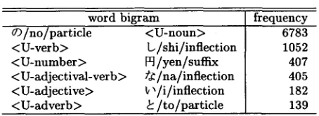
Table 1: Examples of word bigrams including unknown word tags

word bigram frequency

¢)/no/particle <U-verb> <U-number> <U-adjectival-verb> <U-adjective> <U-adverb>

<U-noun> b/shi/inflection H/yen/suffix t~/na/inflection

~/i/inflection /to/particle

6783 1052 407 405 182 139

relative frequencies of the corresponding events in the word segmented training corpus, with appropriate smoothing techniques. T h e maximization search can be efficiently implemented by using the Viterbi- like dynamic programming procedure described in (Nagata, 1994).

2 . 2 M o d i f i c a t i o n t o H a n d l e U n k n o w n W o r d s

To handle unknown words, we made a slight modi- fication in the above word segmentation model. We have introduced unknown word tags for each part of speech t. For example, and <U- verb> represents an unknown noun and an unknown verb, respectively.

If wl is an unknown word whose part of speech is t, the word bigram probability P ( w i [ w l - a ) is approximated as the product of word bigram probability P ( [ w i _ l ) and the probability of wi given it is an unknown word whose part of speech is t, P ( w i [ ) .

P ( w i l w i - 1 ) = P ( l w i - 1 ) P ( w i l , w i - a ) P ( [ w i _ l ) P ( w i l ) (3)

Here, we made an assumption t h a t the spelling of an unknown word solely depends on its part of speech and is independent of the previous word. This is the same assumption made in the hidden Markov model, which is called o u t p u t independence. The probabilities P ( l w i _ l ) can be estimated from the relative frequencies in the training corpus whose infrequent words are replaced with their corresponding unknown word tags based on their part of speeches 2

Table 1 shows examples of word bigrams including unknown word tags. Here, a word is represented by a list of surface form, pronunciation, and part of speech, which are delimited by a slash ' / ' . T h e first

2 Throughout in this paper, we use the term "infrequent words" to represent words that appeared only once in the corpus. They are also called "hapax legomena" or "hapax words". It is well known that the characteristics of hapax legomena are similar to those of unknown words (Baayen and Sproat, 1996).

example " ¢ ) / n o / p a r t i c l e " will appear in the most frequent form of Japanese noun phrases "A © B", which corresponds to "B of A" in English.

As Table 1 shows, word bigrams whose infrequent words are replaced with their corresponding part of speech-based unknown word tags are very i m p o r t a n t information source of the contexts where unknown words appears.

3 U n k n o w n W o r d M o d e l

3 . 1 B a s e l i n e M o d e l

T h e simplest unknown word model depends only on the spelling. We think of an unknown word as a word having a special part of speech . Then, the unknown word model is formally defined as the joint probability of the character sequence wi = cl .. • ck

if it is an unknown word. W i t h o u t loss of generality, we decompose it into the product of word length probability and word spelling probability given its length,

P ( w i [ ) = P ( c x . . . c k [ < V N K > ) =

P ( k I ) P ( c l . . . cklk, ) (4)

where k is the length of the character sequence. We call P ( k I ) the word length model, and

P ( c z . . . ck Ik, ) the word spelling model. In order to estimate the entropy of English, (Brown et al., 1992) approximated P ( k I ) by a Poisson distribution whose p a r a m e t e r is the average word length A in the training corpus, and

P ( c z . . . cklk, ) by the p r o d u c t of character zerogram probabilities. This means all characters in the character set are considered to be selected inde- pendently and uniformly.

)k

P(Cl . . . c k I ) -~ -~. e - ~ p k (5)

where p is the inverse of the number of characters in the character set. If we assume JIS-X-0208 is used as the Japanese character set, p = 1/6879.

Since the Poisson distribution is a single parameter distribution with lower bound, it is appropriate to use it as a first order approximation to the word length distribution. But the Brown model has two problems. It assigns a certain amount of probability mass to zero-length words, and it is too simple to express morphology.

For Japanese word segmentation and OCR error correction, (Nagata, 1996) proposed a modified version of the Brown model. Nagata also assumed the word length probability obeys the Poisson distribution. But he moved the lower bound from zero to one.

()~ - I) k-1

[image:2.612.80.307.113.196.2]

(3)

Instead of zerogram, He approximated the word spelling probability

P(Cl...ck[k,

<UNK>) by the product of word-based character bigram probabilities, regardless of word length.

P(cl... cklk,

<UNK>)

P(Cll<bow> )

YI~=2

P(cilc,_~)P( <eow>lc~)

(7)

where <bow> and <eow> are special symbols that indicate the beginning and the end of a word.

3.2 C o r r e c t i o n o f W o r d Spelling

Probabilities

We find that Equation (7) assigns too little probabilities to long words (5 or more characters). This is because the lefthand side of Equation (7) represents the probability of the string

cl ... Ck

in the set of all strings whose length are k, while the righthand side represents the probability of the string in the set of all possible strings (from length zero to infinity).

Let

Pb(cz

...ck]<UNK>) be the probability of character string Cl...ck estimated from the character bigram model.

Pb(cl...

ckI<UNK>) --

P(Cl]<bow>)

1-I~=2 P(c~lc,-1)P( <e°w>lck)

(8)

Let Pb (kl <UNK>) be the sum of the probabilities of all strings which are generated by the character bigram model and whose length are k. More appropriate estimate for

P(cl... cklk,

<UNK>) is,

P(cl... cklk,

<UNK>) ~ Pb(cl ... ckI<UNK>)

Pb(kI<UNK>)

(9)

But how can we estimate

Pb(kI<UNK>)?

It is difficult to compute it directly, but we can get a rea- sonable estimate by considering the unigram case.

If strings are generated by the character unigram model, the sum of the probabilities of all length k strings equals to the probability of the event that the end of word symbol <eow> is selected after a character other than <eow> is selected k - 1 times.

Pb(k[<UNK>) ~ (1

-P(<eow>))k-ZP(<eow>)(10)

Throughout in this paper, we used Equation (9) to compute the word spelling probabilities.

3.3 J a p a n e s e O r t h o g r a p h y a n d W o r d L e n g t h D i s t r i b u t i o n

In word segmentation, one of the major problems of the word length model of Equation (6) is the decomposition of unknown words. When a substring of an unknown word coincides with other word in the dictionary, it is very likely to be decomposed into the dictionary word and the remaining substring. We find the reason of the decomposition is that the word

0.5

0.45

0.4

0.35

0.3

0.25

0.2

0.15

0.1

0.05

0

Word Length Distribution

, i i

Probs from Raw Counts (hapax words) Estimates by Poisson (hapax words) -+---

/ /

I I i i

2 4 6 8 10

Word Character Length

Figure 1: Word length distribution of unknown words and its estimate by Poisson distribution

0.5

0.45

0 . 4

035

0.3

0.25

0.2

0.15

0.1

0.05

0 0

Unknown Word Length Oistflbutlon

kanJl katakana ~

2 4 6 8 10

Word Character Length

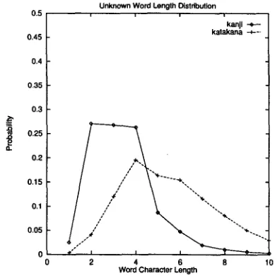
Figure 2: Word length distribution of

kanji

words and

katakana

words

length model does not reflect the variation of the word length distribution resulting from the Japanese orthography.

Figure 1 shows the word length distribution of infrequent words in the EDR corpus, and the estimate of word length distribution by Equation (6) whose parameter (A = 4.8) is the average word length of infrequent words. The empirical and the estimated distributions agree fairly well. But the estimates by Poisson are smaller than empirical probabilities for shorter words ( < = 4 characters), and larger for longer words (> characters). This is because we rep-

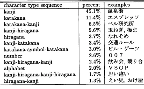
[image:3.612.319.510.81.278.2] [image:3.612.317.513.338.533.2]

(4)

Table 2: C h a r a c t e r t y p e configuration of infrequent words in the E D R corpus

Table 3: Examples of c o m m o n character bigrams for each p a r t of speech in the infrequent words

character type sequence kanji

katakana katakana-kanji kanji-hiragana hiragana kanji-katakana

kat akana-symbol-katakana number

kanji-hiragana-kanji alphabet

kanji-hir agana-kanji-hir agana hiragana-kanji

percent 45.1% 11.4% 6.5% 5.6% 3.7% 3.4% 3.0% 2.6% 2.4% 2.0% 1.7%

1.3%

examples

=~y~T'I/y Y

t . * a g , ~ $

OO7 ~ , ~ V ~

V S O P

± ~ , ~ , ~ ~-~,~!

resented all unknown words by one length model. Figure 2 shows the word length distribution of words consists of only

kanji

characters and words consists of only

katakana

characters. It shows t h a t the length of

kanji

words distributes around 3 characters, while t h a t of

katakana

words distributes around 5 characters. T h e empirical word length distribution of Figure 1 is, in fact, a weighted sum of these two distributions.

In the J a p a n e s e writing system, there are at least five different types of characters other t h a n punc- tuation marks:

kanji, hiragana, katakana,

R o m a n alphabet, and Arabic numeral.

Kanji

which means 'Chinese character' is used for b o t h Chinese origin words and J a p a n e s e words semantically equivalent to Chinese characters.

Hiragana

and

katakana

are syllabaries: T h e former is used primarily for gram- matical function words, such as particles and inflec- tional endings, while the latter is used primarily to transliterate Western origin words. R o m a n a l p h a b e t is also used for Western origin words and acronyms. Arabic numeral is used for numbers.

Most J a p a n e s e words are written in

kanji,

while more recent loan words are written in

katakana.

Katakana

words are likely to be used for technical terms, especially in relatively new fields like c o m p u t e r science.

Kanji

words are shorter t h a n

katakana

words because

kanji

is based on a large ( > 6,000) alphabet of ideograms while

katakana

is based on a small (< 100) a l p h a b e t of phonograms.

Table 2 shows the distribution of character t y p e sequences t h a t constitute the infrequent words in the E D R corpus. It shows a p p r o x i m a t e l y 65% of words are constituted by a single character type. Among the words t h a t are constituted by more t h a n two character types, only the kanji-hiragana and hiragana-kanji sequences are m o r p h e m e s and others are c o m p o u n d words in a strict sense although they

p a r t of speech character b i g r a m frequency noun

n u m b e r adjectival-verb verb

adjective adverb

< e o w > 1

< e o w > ~'J < e o w > b < e o w > 0 < e o w >

1343 484 327 213 69 63

are identified as words in the E D R corpus 3

Therefore, we classified J a p a n e s e words into 9 word types based on the character types t h a t consti- t u t e a word: < s y m > , < n u m > , < a l p h a > , < h i r a > , < k a t a > , and < k a n > represent a sequence of symbols, numbers, alphabets,

hiraganas, katakanas,

and

kanjis,

respectively. < k a n - h i r a > and < h i r a - k a n > represent a sequence of

kanjis

followed by

hiraganas

a n d t h a t of

hiraganas

followed by

kanjis,

respectively. T h e rest are classified as < m i s c > .

T h e resulting unknown word model is as follows. We first select the word type, then we select the length and spelling.

P(Cl ...ckI<UNK>)

=

P( <WT>I<UNK> )P(kI<WT> ,

d U N K > )

P(cl... cklk,

< W T > , ) (11)

3.4 P a r t o f S p e e c h a n d W o r d M o r p h o l o g y It is obvious t h a t the beginnings a n d endings of words play an i m p o r t a n t role in tagging p a r t of speech. Table 3 shows examples of c o m m o n character bigrams for each p a r t of speech in the infrequent words of the E D R corpus. T h e first example in Table 3 shows t h a t words ending in ' - - ' are likely to be nouns. This symbol typically a p p e a r s at the end of transliterated Western origin words written in

katakana.

It is n a t u r a l to m a k e a model for each p a r t of speech. T h e resulting unknown word model is as follows.

P(Cl .. • c k ] ) =

P(k]<U-t>)P(Cl... cklk,

) (12)

By introducing the distinction of word t y p e to the model of Equation (12), we can derive a more sophis- ticated unknown word model t h a t reflects b o t h word

[image:4.612.79.316.123.270.2]

(5)

type and part of speech information. This is the unknown word model we propose in this paper. It first selects the word type given the part of speech, then the word length and spelling.

P(cl...

c l<U-t>) =

P( <WT>I<U-t> )P(kI<WT>,

<U-t>)

P(Cl... cklk,

< W T > , <U-t>) (13)

Table 4: The amount of training and test sets

sentences word tokens char tokens

training set 100,000 2,460,188 3,897,718

test set-1 test set-2 100,000 5,000 2,465,441 122,064 3,906,260 192,818

The first factor in the righthand side of Equa- tion (13) is estimated from the relative frequency of the corresponding events in the training corpus.

p ( < W T > I ) = C ( < W T > , <U-t>) C(<U-t>) (14)

Here, C(.) represents the counts in the corpus. To estimate the probabilities of the combinations of word type and part of speech that did not appeared in the training corpus, we used the Witten-Bell method (Witten and Bell, 1991) to obtain an estimate for the sum of the probabilities of unobserved events. We then redistributed this evenly among all unobserved events a

The second factor of Equation (13) is estimated from the Poisson distribution whose parameter

'~<WT>,<U-t>

is the average length of words whose word type is < W T > and part of speech is <U-t>.

P ( k I < W T > , <U-t>) =

( ) ~ < W W > , - l ) u-1 e - - ( A < W W > , - l ) (15) (k-l)!

If the combinations of word type and part of speech that did not appeared in the training corpus, we used the average word length of all words.

To compute the third factor of Equation (13), we have to estimate the character bigram probabilities that are classified by word type and part of speech. Basically, they are estimated from the relative frequency of the character bigrams for each word type and part of speech.

f(cilci-1,

< W T > , <U-t>) =

C ( < W T > , , c i _ 1 ,cl)

C(<WT>,<U-t>,ci_l) (16)

However, if we divide the corpus by the combination of word type and part of speech, the amount of each training data becomes very small. Therefore, we linearly interpolated the following five probabilities (Jelinek and Mercer, 1980).

P(c~lci_l,

< W T > , <U-t>) =

4 T h e W i t t e n - B e l l m e t h o d e s t i m a t e s t h e p r o b a b i l i t y of ob- s e r v i n g novel e v e n t s to be r/(n+r), w h e r e n is t h e t o t a l n u m - b e r of e v e n t s s e e n previously, a n d r is t h e n u m b e r of s y m b o l s t h a t are d i s t i n c t . T h e p r o b a b i l i t y o f t h e e v e n t o b s e r v e d c t i m e s is c/(n + r).

oqf(ci,

< W T > , <U-t>)

+ a 2 f ( c i 1Ci-1, < W T > , <U-t>)

+a3f(ci) +

aaf(cilci_,) +

~5(1/V) (17)

Where

~1+(~2+~3+cq+c~5 --- 1.

f(ci,

< W T > , <U-t>) and

f(ci[ci-t,

< W T > , <U-t>) are the relative frequencies of the character unigram and bigram for each word type and part of speech,

f(ci) and f(cilci_l)

are the relative frequencies of the character unigram and bigram. V is the number of characters (not

to-

kens

but

types)

appeared in the corpus.

4 E x p e r i m e n t s

4.1 T r a i n i n g a n d Test D a t a for t h e Language M o d e l

We used the EDR Japanese Corpus Version 1.0 (EDR, 1991) to train the language model. It is a manually word segmented and tagged corpus of ap- proximately 5.1 million words (208 thousand sentences). It contains a variety of Japanese sentences taken from newspapers, magazines, dictionaries, en- cyclopedias, textbooks, etc..

In this experiment, we randomly selected two sets of 100 thousand sentences. The first 100 thousand sentences are used for training the language model. The second 100 thousand sentences are used for test- ing. The remaining 8 thousand sentences are used as a heldout set for smoothing the parameters.

For the evaluation of the word segmentation accuracy, we randomly selected 5 thousand sentences from the test set of 100 thousand sentences. We call the first test set (100 thousand sentences) "test set-l" and the second test set (5 thousand sentences) "test set-T'. Table 4 shows the number of sentences, words, and characters of the training and test sets.

There were 94,680 distinct words in the training test. We discarded the words whose frequency was one, and made a dictionary of 45,027 words. Af- ter replacing the words whose frequency was one with the corresponding unknown word tags, there were 474,155 distinct word bigrams. We discarded the bigrams with frequency one, and the remaining 175,527 bigrams were used in the word segmentation model.

As for the unknown word model, word-based character bigrams are computed from the words with

(6)

Table 5: Cross entropy (CE) per word and character perplexity (PP) of each unknown word model

unknown word model CE per word char PP

Poisson+zerogram 59.4 2032

Poisson+bigram 37.8 128

WT+Poisson+bigram 33.3 71

frequency one (49,653 words). There were 3,120 distinct character unigrams and 55,486 distinct character bigrams. We discarded the bigram with frequency one and remaining 20,775 bigrams were used. There were 12,633 distinct character unigrams and 80,058 distinct character bigrams when we classified them for each word type and part of speech. We discarded the bigrams with frequency one and remaining 26,633 bigrams were used in the unknown word model.

Average word lengths for each word type and part of speech were also computed from the words with frequency one in the training set.

4.2 Cross E n t r o p y a n d P e r p l e x i t y

Table 5 shows the cross entropy per word and character perplexity of three unknown word model. The first model is Equation (5), which is the combination of Poisson distribution and character zerogram (Poisson + zerogram). The second model is the combination of Poisson distribution (Equation (6)) and character bigram (Equation (7)) (Poisson + bigram). The third model is Equation (11), which is a set of word models trained for each word type (WT + Poisson + bigram). Cross entropy was computed over the words in test set-1 that were not found in the dictionary of the word segmentation model (56,121 words). Character perplexity is more intu- itive than cross entropy because it shows the average number of equally probable characters out of 6,879 characters in JIS-X-0208.

Table 5 shows that by changing the word spelling model from zerogram to big-ram, character perplexity is greatly reduced. It also shows that by making a separate model for each word type, character perplexity is reduced by an additional 45% (128 -~ 71). This shows that the word type information is useful for modeling the morphology of Japanese words.

4.3 P a r t of S p e e c h P r e d i c t i o n A c c u r a c y w i t h o u t C o n t e x t

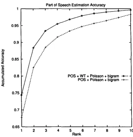
Figure 3 shows the part of speech prediction accuracy of two unknown word model without context. It shows the accuracies up to the top 10 candidates. The first model is Equation (12), which is a set of word models trained for each part of speech (POS + Poisson + bigram). The second model is Equa- tion (13), which is a set of word models trained for

Part of Speech Estimation Accuracy

0.95 ~"~ . . . ~ ' * * " " 0.9 / ' " "

0.85

0.8 ~- / ~ + WT + Poisson + bigram -e--

N I//

POS + Poisson + bigram --~---

0.75 [ /

0.65

1 2 3 4 5 6 7 8 9 10 Rank

Figure 3: Accuracy of part of speech estimation

each part of speech and word type (POS + WT + Poisson + bigram). The test words are the same 56,121 words used to compute the cross entropy.

Since these unknown word models give the probability of spelling for each part of speech

P(wlt),

we used the empirical part of speech probability

P(t)

to compute the joint probability

P(w, t).

The part of speech t that gives the highest joint probability is selected.

= argmtaxP(w,t ) = P(t)P(wlt )

(18)

The part of speech prediction accuracy of the first and the second model was 67.5% and 74.4%, respectively. As Figure 3 shows, word type information improves the prediction accuracy significantly.

4.4 W o r d S e g m e n t a t i o n A c c u r a c y

Word segmentation accuracy is expressed in terms of recall and precision as is done in the previous research (Sproat et al., 1996). Let the number of words in the manually segmented corpus be Std, the number of words in the output of the word segmenter be Sys, and the number of matched words be M.

Recall

is defined as M/Std, and

precision

is defined as M/Sys. Since it is inconvenient to use both recall and precision all the time, we also use the F-measure to indicate the overall performance. It is calculated

by

F = (f~2+l.0) x P x R

f~2 x P + R (19)

[image:6.612.322.540.81.306.2]

(7)

Table 6: Word segmentation accuracy of all words

rec prec F Poisson+bigram 94.5 9 3 . 1 93.8 WT+Poisson+bigram 94.4 93.8 94.1 POS+Poisson+bigram 94.4 93.6 94.0 POS+WT+Poisson+bigram 94.6 93.7 94.1

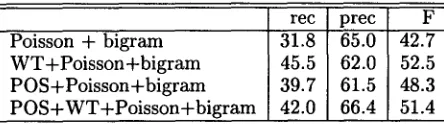
Table 7: Word segmentation accuracy of unknown words

64.1%.

Other than the usual recall/precision measures, we defined another precision (prec2 in Table 8), which roughly correspond to the tagging accuracy in English where word segmentation is trivial. Prec2 is defined as the percentage of correctly tagged unknown words to the correctly segmented unknown words. Table 8 shows that tagging precision is improved from 88.2% to 96.6%. The tagging accuracy in context (96.6%) is significantly higher than that without context (74.4%). This shows that the word bigrams using unknown word tags for each part of speech are useful to predict the part of speech.

rec prec F Poisson + bigram 31.8 65.0 42.7 WT+Poisson+bigram 45.5 62.0 52.5 POS+Poisson+bigram 39.7 61.5 48.3 POS+WT+Poisson+bigram 42.0 66.4 51.4

f~ = 1.0 throughout this experiment. That is, we put equal importance on recall and precision.

Table 6 shows the word segmentation accuracy of four unknown word models over test set-2. Com- pared to the baseline model (Poisson + bigram), by using word type and part of speech information, the precision of the proposed model (POS + WT + Pois- son + bigram) is improved by a modest 0.6%. The impact of the proposed model is small because the out-of-vocabulary rate of test set-2 is only 3.1%.

To closely investigate the effect of the proposed unknown word model, we computed the word segmentation accuracy of unknown words. Table 7 shows the results. The accuracy of the proposed model (POS + WT + Poisson + bigram) is significantly higher than the baseline model (Poisson + bigram). Recall is improved from 31.8% to 42.0% and precision is improved from 65.0% to 66.4%.

Here, recall is the percentage of correctly segmented unknown words in the system output to the all unknown words in the test sentences. Precision is the percentage of correctly segmented unknown words in the system's output to the all words that system identified as unknown words.

Table 8 shows the tagging accuracy of unknown words. Notice that the baseline model (Poisson + bigram) cannot predict part of speech. To roughly estimate the amount of improvement brought by the proposed model, we applied a simple tagging strat- egy to the output of the baseline model. That is, words that include numbers are tagged as numbers, and others are tagged as nouns.

Table 8 shows that by using word type and part of speech information, recall is improved from 28.1% to 40.6% and precision is improved from 57.3% to

5 R e l a t e d W o r k

Since English uses spaces between words, unknown words can be identified by simple dictionary lookup. So the topic of interest is part of speech estimation. Some statistical model to estimate the part of speech of unknown words from the case of the first letter and the prefix and suffix is proposed (Weischedel et al., 1993; Brill, 1995; Ratnaparkhi, 1996; Mikheev, 1997). On the contrary, since Asian languages like Japanese and Chinese do not put spaces between words, previous work on unknown word problem is focused on word segmentation; there are few studies estimating part of speech of unknown words in Asian languages.

The cues used for estimating the part of speech of unknown words for Japanese in this paper are basically the same for English, namely, the prefix and suffix of the unknown word as well as the previous and following part of speech. The contribution of this paper is in showing the fact that different character sets behave differently in Japanese and a better word model can be made by using this fact.

By introducing different length models based on character sets, the number of decomposition errors of unknown words are significantly reduced. In other words, the tendency of over-segmentation is cor- rected. However, the spelling model, especially the character bigrams in Equation (17) are hard to estimate because of the data sparseness. This is the main reason of the remaining under-segmented and over-segmented errors.

To improve the unknown word model, feature- based approach such as the maximum entropy method (Ratnaparkhi, 1996) might be useful, because we don't have to divide the training data into several disjoint sets (like we did by part of speech and word type) and we can incorporate more lin- guistic and morphological knowledge into the same probabilistic framework. We are thinking of re- implementing our unknown word model using the maximum entropy method as the next step of our research.

[image:7.612.62.286.112.173.2] [image:7.612.64.286.241.303.2]

(8)

Table 8: Part of speech tagging accuracy of unknown words (the last column represents the percentage of correctly tagged unknown words in the correctly segmented unknown words)

rec prec F prec2

Poisson+bigram 28.1 57.3 37.7 88.2

WT+Poisson+bigram 37.7 51.5 43.5 87.9

POS+Poisson+bigram 37.5 58.1 45.6 94.3

POS+WT+Poisson+bigram 40.6 64.1 49.7 96.6

6 C o n c l u s i o n

We present a statistical model of Japanese unknown words using word morphology and word context. We find that Japanese words are better modeled by clas- sifying words based on the character sets (kanji, hi- ragana, katakana, etc.) and its changes. This is because the different character sets behave differently in many ways (historical etymology, ideogram vs. phonogram, etc.). Both word segmentation accuracy and part of speech tagging accuracy are improved by treating them differently.

R e f e r e n c e s

Harald Baayen and Richard Sproat. 1996. Estimat- ing lexical priors for low-frequency morphologi- cally ambiguous forms. Computational Linguis- tics, 22(2):155-166.

Eric Brill. 1995. Transformation-based error-driven learning and natural language processing: A case study in part-of-speech tagging. Computational Linguistics, 21(4):543-565.

Peter F. Brown, Stephen A. Della Pietra, Vincent J. Della Pietra, Jennifer C. Lal, and Robert L. Mercer. 1992. An estimate of an upper bound for the entropy of English. Computational Linguis- tics, 18(1):31-40.

Jing-Shin Chang, Yi-Chung Lin, and Keh-Yih Su. 1995. Automatic construction of a Chinese electronic dictionary. In Proceedings of the Third Workshop on Very Large Corpora, pages 107-120. EDR. 1991. EDR electronic dictionary version 1 technical guide. Technical Report TR2-003, Japan Electronic Dictionary Research Institute. Pascale Fung and Dekai Wu. 1994. Statistical aug-

mentation of a Chinese machine-readable dictionary. In Proceedings of the Second Workshop on

Very Large Corpora, pages 69-85.

Masahiko Haruno and Yuji Matsumoto. 1997. Mistake-driven mixture of hierachical tag context trees. In Proceedings of the 35th ACL and 8th EA CL, pages ~ 230-237.

F. Jelinek and R. L. Mercer. 1980. Interpolated estimation of Markov source parameters from sparse data. In Proceedings of the Workshop on Pattern Recognition in Practice, pages 381-397.

Andrei Mikheev. 1997. Automatic rule induction for unknown-word guessing. Computational Linguis- tics, 23(3):405-423.

Shinsuke Mori and Makoto Nagao. 1996. Word ex- traction from corpora and its part-of-speech estimation using distributional analysis. In Proceed- ings of the 16th International Conference on Com- putational Linguistics, pages 1119-1122.

Masaaki Nagata. 1994. A stochastic Japanese morphological analyzer using a forward-dp backward- A* n-best search algorithm. In Proceedings of the 15th International Conference on Computational Linguistics, pages 201-207.

Masaaki Nagata. 1996. Context-based spelling correction for Japanese OCR. In Proceedings of the 16th International Conference on Computational Linguistics, pages 806-811.

Adwait Ratnaparkhi. 1996. A maximum entropy model for part-of-speech tagging. In Proceedings of Conference on Empirical Methods in Natural Language Processing, pages 133-142.

Richard Sproat, Chilin Shih, William Gale, and Nancy Chang. 1996. A stochastic finite-state word-segmentation algorithm for Chinese. Com- putational Linguistics, 22(3):377-404.

Koichi Takeuchi and Yuji Matsumoto. 1997. HMM parameter learning for Japanese morphological analyzer. Transaction of Information Processing of Japan, 38(3):500-509. (in Japanese).

Ralph Weischedel, Marie Meteer, Richard Schwartz, Lance Ramshaw, and Jeff Palmucci. 1993. Cop- ing with ambiguity and unknown words through probabilistic models. Computational Linguistics,

19(2):359-382.

Ian H. Witten and Timothy C. Bell. 1991. The zero-frequency problem: Estimating the probabilities of novel events in adaptive text compres- sion. IEEE Transaction on Information Theory, 37(4):1085-1094.