Munich Personal RePEc Archive
Uncertainty, Learning, and Local
Opposition to Hydraulic Fracturing
Hess, Joshua and Manning, Dale and Iverson, Terry and
Cutler, Harvey
Department of Economics; University of South Carolina,
Department of Agricultural Resource Economics; Colorado State
University, Department of Economics: Colorado State University
30 December 2016
Online at
https://mpra.ub.uni-muenchen.de/79238/
1
Uncertainty, Learning, and Local Opposition to Hydraulic Fracturing
Joshua H. Hess1,*, Dale T. Manning2, Terry Iverson3, Harvey Cutler3
December 2016
Abstract
The development of oil and gas extraction technologies, including hydraulic fracturing (fracking), has increased fossil fuel reserves in the US. Despite benefits, uncertainty over environmental damages has led to fracking bans, both permanent and temporary, in many
jurisdictions. We develop a stochastic dynamic learning model parameterized with a computable general equilibrium model to explore if uncertainty about damages, combined with the ability to learn about risks, can explain fracking bans in practice. Applying the model to a representative Colorado municipality, we quantify the quasi-option value (QOV), which creates an additional incentive to ban fracking temporarily in order to learn, though it only influences policy in a narrow range of oil and gas prices. To our knowledge, this is the first attempt to quantify an economy-wide QOV associated with a local environmental policy decision.
JEL: C61, C68, Q38, Q58
Keywords: hydraulic fracturing; quasi-option value; stochastic dynamic program; computable general equilibrium model
1 Department of Economics; University of South Carolina * Corresponding author: josh.h.hess@gmail.com
2
1. Introduction
New technologies for extracting oil and gas from shale deposits—most importantly, hydraulic
fracturing (fracking)—have greatly increased fossil fuel reserves across the United States and
beyond. While these innovations have the potential to bring substantial economic benefits
(Hausman and Kellogg 2015), they also have the potential to create environmental costs
(Muehlenbachs et al. 2015, Krupnick and Gordon 2015, Hill 2013). Many jurisdictions have
temporarily banned fracking (e.g., Longmont, CO; New York State; Germany), despite, in some
cases, seemingly positive expected net local benefits (Wobbekind et al., 2014). Plausibly, such
bans stem from the high degree of uncertainty about potential harm, together with the
opportunity to learn from experiences elsewhere during the ban. Of course, this is a classic
quasi-option value story applied to a situation in which a novel technology gives rise to uncertain
environmental risks.
Our goal in this paper is to develop a framework that can be used to quantify the quasi-option
value (QOV) and assess its importance to the prevalence of fracking bans in practice. To do this,
we develop a methodology for linking an empirically grounded computable general equilibrium
(CGE) model with a dynamic QOV model, allowing for a data-driven estimation of the QOV
associated with a real-world environmental policy choice. Since fracking affects many agents
within a community, a CGE model that quantifies economy-wide consumption impacts over time
provides the information needed to evaluate a potential ban. Solving a dynamic program
containing a large-dimensional CGE presents a substantial numerical challenge, but we
overcome it by assuming that local fracking benefits are additively separable from uncertain
fracking damages. Under this assumption, we are able to solve the model by running the CGE
3
to a finite-time, stochastic dynamic program with Bayesian learning. The methodology
developed here is one of the first to place a numerical value on the economy-wide QOV
associated with learning about local environmental damages.
By choosing to implement a temporary ban, policymakers delay fracking benefits but learn about
the true magnitude of fracking damages from an informative, though noisy, signal. Allowing
fracking brings economic benefits with uncertain, potentially irreversible, damages. The
framework allows for the quantification of the economy-wide, and hence social, quasi-option
value that arises from the preservation of the option to avoid irreversible environmental damages.
It also permits consideration of additional factors that influence the economic decision to
develop unconventional plays, including the value of local oil and gas reserves.
We parameterize the model to match a representative municipality in the US state of Colorado.
In this setting, despite positive expected economy-wide net benefits from fracking, a ban can be
rationalized at current oil prices4 if the learning process is sufficiently precise. Results indicate
that a one-period reduction in the time required to reduce the variance of uncertain
environmental damages by half is, on average, equivalent to a $1 per barrel increase in the price
of oil. This suggests that while the ability to learn can influence optimal policy choices, the value
of local reserves likely plays a larger role. Nevertheless, increasing the precision of future
information about fracking damages increases the likelihood of a ban in initial periods; though
after this initial ban, policymakers allow fracking more frequently when it is beneficial and
continue banning when it is not.
4
4
The ability to delay and revisit an uncertain and irreversible decision with better information is
valuable (Arrow and Fischer 1974, Henry 1974, Hanemann 1988, Dixit and Pindyck 1994).
Traeger (2014) defines the QOV as the value of learning, conditional on the ability to postpone a
decision. Yet, to our knowledge, an economy-wide QOV has not been quantified in an applied
policy setting.
For the most part, the existing economics literature on fracking focuses on either benefits or
costs. Fracking benefits include increased employment (Weber 2012; Maniloff and
Mastromonaco 2015), welfare improvements for producers and consumers of natural gas
(Hausman and Kellogg 2015), and revenues to mineral rights owners (Brown and Fitzgerald).
Others have investigated fracking burdens (Krupnick, Wang, and Wang 2014; Krupnick and
Gordon 2015), including property value impacts (Muehlenbachs, Spiller, and Timmins 2015) and
health effects (Chen, et al. 2000; Aguilera et al. 2009; Slama et al., 2009; Hill 2013). Hedonic
analyses of fracking impacts on property values can also provide a means to capture net fracking
impacts (Gopalakrishnan and Klaiber 2014; Bennett and Loomis 2015). Our contribution, in
contrast, builds on the prior literatures on fracking benefits and costs, while embedding a local
fracking policy decision within an explicit decision-theoretic framework. To our knowledge, this
analysis is the first to quantify the value of learning about the full costs of fracking in practice,
and the first to carefully assess the economic rationale for observed bans.
The rest of the paper is organized as follows. Section 2 provides an overview of fracking bans in
practice and reviews the literature on fracking and option values. Section 3 introduces the model
and Section 4 discusses our parameterized application and economic assumptions. Section 5
5
2. Related Literature and Background
This section begins with an overview of local opposition to fracking5. We then describe the
current literature on the economic benefits of fracking and the uncertain damages. Finally, we
relate the current paper to the literature on uncertainty and learning in environmental economics.
2.1 Fracking Bans
Fracking bans in the US began in November 2010 when Pittsburg implemented a city-wide ban.
Buffalo, NY followed with a largely symbolic ban in February 2011. Dryden, NY then enacted a
ban in August 2011 and became a center of legal contention, though the ban held up in court.
Emboldened by Dryden’s success, several New York towns6 enacted or adopted bans,
culminating in a statewide ban issued by Governor Cuomo in December 2014. Vermont, which
has no oil and gas development, banned fracking in March of 2012, and Connecticut enacted a
three-year ban on storage and handling of fracking waste in August 2014. Other bans in large US
cities include Los Angeles and Beverly Hills in CA, Philadelphia, PA, and Denton, TX7, though
on May 2015, the State of Texas made local bans illegal. Denton overturned its ban the
following month.
A similar battle occurred on the Colorado Front Range, which sits atop the Niobrara shale
formation. The town of Longmont changed its charter to prohibit fracking in November 2012
and was sued by the Colorado Oil and Gas Association – a large industry group – alongside the
principal development interest, TOP Operating, and the Colorado Oil and Gas Conservation
Commission, the state agency in charge of regulation. Seemingly unfazed by this litigation, the
cities of Fort Collins, Lafayette, Boulder, and Broomfield passed similar measures in November
5
A list of fracking bans in practice can be found at http://www.foodandwaterwatch.org
6
Syracuse, Albany, Woodstock, Rochester, Wawarsing, Kirkland, and Canandaigua 7
6
2013. On May 2, 2016, however, the Colorado Supreme Court ruled in favor of the State’s
rights, overturning the Longmont ban and the Fort Collins moratorium8.
Mora County, NM became the first US County to have a ban in May 2013, but a federal judge
overturned it in January 2015. Hawaii County enacted a ban in October of 2013 and was
followed by three California counties: Santa Cruz County in May 2014 and then Mendocino and
San Benito Counties in November elections that year.
Internationally, France became the first country with a moratorium in June 20119. Since then,
Bulgaria, Luxembourg, Germany, Scotland, and Wales have banned fracking. In addition, due to
concerns about local environmental impacts, the Cantabria Region of Spain, Nova Scotia,
Quebec, and Five City Breaks municipality of Argentina have implemented fracking bans.
Boudet et al. (2014) argue that fracking bans accompany a high degree of public uncertainty
about local damages. A 2012 Pew Center poll found that 26% of Americans had heard a lot
about fracking, 37% had heard a little, and 37% had heard nothing. Regardless of the level of
information, it is perceptions about risk (informed or otherwise) that drive local policy. Graham
et al. (2014) find that the public is most concerned about water quality and seismic activity,
despite a general scientific consensus that best practices manage these particular risks well.
2.2 Economic Benefits of Fracking
While it is obvious that exploiting valuable fossil fuel reserves will confer economic value, it is
less clear how much of the created value will accrue to the local economy where fracking occurs.
Hausman and Kellogg (2015) use an econometric approach and find economy-wide total surplus
8
http://www.nytimes.com/2016/05/03/us/colorado-court-strikes-down-local-bans-on-fracking.html 9
7
gains of a third of a percent in the US. Regionally focused work has estimated significant
employment gains – ex ante – to Pennsylvania (Considine et al. 2010), Colorado (Wobbekind et
al. 2014), and Arkansas (CBER 2008). However, these studies use input-output models and
results are sensitive to assumptions about household spending and savings behavior, labor supply
elasticity, and mineral rights ownership. This means that benefits are likely to be significantly
overstated (Kinnaman 2011). More recent ex post analyses find much smaller employment
impacts than ex ante predictions (Weber 2012). Maniloff and Mastromonaco (2015) find that ex
post job growth fell ‘well short’ of ex ante predictions. Furthermore, there is a debate as to the
persistence of economic benefits in so-called ‘boom towns’ (Allcott and Keniston 2011;
Jacobsen and Parker 2014). Contrary to previous findings by Allcott and Keniston (2011),
Maniloff and Mastomonaco (2015) find evidence of increases in manufacturing wages which
could harm the competitiveness of non-resource sectors.
In the model developed here, local fracking benefits are captured using a calibrated CGE model
that includes oil and gas production. The portion of benefits that accrue locally follows from our
assumptions about nonlocal resource ownership.
2.3 Fracking Damages
Despite a consensus that risks exist, there remain significant gaps in the literature connecting risk
pathways to economic impacts (Jackson et al. 2014; Shonkoff et al. 2014). Krupnick and Gordon
(2015) prescribe important pathways through which routine fracking activities may impact
humans and the environment. Examples include habitat disruption, groundwater contamination,
8
215 experts from industry, academia, government, and NGOs finds a high degree of consensus
concerning the most important pathways that arise during normal fracking activities.
Hedonic property valuation studies have attempted to quantify the cost of these local impacts
(Boxall, et al. 2005; Gopalakrishnan and Klaiber 2014). Typically, these studies find negative
impacts on housing values from nearby oil and gas development, especially if the home depends
on groundwater (Muehlenbachs, Spiller, and Timmins 2015). Bennett and Loomis (2015)
estimate that each well drilled within a half-mile of a house in Weld County, Colorado decreases
the home value by $1,805 in urban areas.
Many human health studies have focused on benzene pollution10 outside the fracking context
(Chen, et al. 2000; Aguilera et al. 2009; Slama et al., 2009; Zahran et al. 2012) and have
highlighted significant health damages, including low birth weight. Hill (2013) shows that
fracking in Pennsylvania increased the occurrence of low birth weight (by 25%) and term birth
weight (by 18%). She estimates a lower bound of the public cost to be $4.1 million due to low
infant birth weights caused by benzene air pollution from fracking in Pennsylvania in 2010.
2.4 Learning about Environmental Risks
Weisbrod (1964) initiated the irreversible decision literature. Arrow and Fisher (1974) and Henry
(1974) develop the use of the quasi-option value in the environmental and resource economics
literature, and Hanemann (1989) formalizes the notion into what is now commonly called the
Arrow-Fisher-Hanemann-HenryQuasi-Option Value (QOV). A similar concept, the real options
approach, developed independently in the finance literature. Pindyck (1991) shows its usefulness
10
9
in a dynamic programming application, and Dixit and Pindyck (1994) bring the real options
approach to the mainstream environmental and resource economics literature. Mensink and
Requate (2005) point out that the Dixit and Pindyck option value (DPOV) and the QOV are not
necessarily equivalent. Specifically, they find that when postponement is initially beneficial and
the net present value of a project is strictly positive, the DPOV captures the QOV in addition to
the value created from doing the project in a later period in the absence of learning.
Traeger (2014) extends Mensink and Requate (2005) and provides a general relationship
between QOV and DPOV: the QOV is the value of learning conditional on postponement and
the DPOVis the net value of postponement under learning. The literature proves two important
properties of the QOV that are relevant to our model. Arrow and Fisher (1974) show that the
QOV is increasing in prior uncertainty in the special case of linear net benefits (although
Hanemann (1989) demonstrates that this does not hold in general). Second, Hanemann (1989)
shows that the QOV increases as future information becomes more precise. These properties
imply that high uncertainty and fast learning increase the QOV, making a temporary ban more
likely.
QOV models are routinely applied to climate policy. Chichilnisky and Heal (1993) argue that the
failure of global warming models to account for irreversibility has led to an understated need for
immediate action, though Ulph and Ulph (1997) show that Epstein’s (1980) irreversibility
conditions are not met for even a simple, two-period model of global warming. Kolstad (1996a)
jointly examines capital investment in abatement (sunk-cost irreversibility) and environmental
damages from the stock of carbon (emissions irreversibility) and argues that either sufficiently
10
(1996b) concludes that capital investment irreversibility increases initial optimal emissions levels
(lowers abatement). Fisher and Narain (2003) support this result, finding that the negative effect
of capital irreversibility on optimal abatement outweighs the impact of irreversible
environmental damages. Lemoine and Traeger (2014) model irreversible changes in climate
sensitivity as an unknown threshold is crossed, but learning is strictly ex post in their model.
They find that the existence of ‘tipping points’ raises the optimal first-period carbon tax.
Learning models in which policymakers make a path of decisions over time have also been
widely applied in the resource economics literature (Walters 1986; Holling and Meffe 1996;
Thrower and Martinez 2000; Prato 2005; Bond and Loomis 2009) and in the climate change
literature (Kelly and Kolstad 1999; Karp and Zhang 2006; Leach 2007; Jensen and Traeger 2013;
Traeger 2015). In this case, small changes to policy act as experiments that impact both stocks
(resource, capital, carbon, etc.) and information about the uncertain factor (e.g., nature’s
response, price, temperature). In models of this form, known as open-loop or adaptive-loop
models, consequences are not necessarily irreversible. Then, the ability to learn incentivizes a
more aggressive initial policy when the benefits of obtaining information outweigh the costs.
A notable exception to this result is Jensen and Traeger (2013). This model incorporates
normally distributed Bayesian learning about uncertain climate sensitivity and stochastic
temperature increases, which determines both the rate of learning and expected damages.
Interestingly, when the rate of learning becomes stochastic – and signals are less informative –,
the impact of juxtaposing uncertainty and learning is to increase optimal carbon abatement, even
11
We model the decision to ban fracking as an irreversible decision in a context of uncertainty and
learning for three reasons. First, in practice, fracking is a relatively new technology and little is
known about it11. This uncertainty becomes resolved over time as the industry learns best
practices, as municipalities learn how to regulate, as the public becomes familiar with the
technology, and as the body of scientific analysis grows. Second, the decision to frack for most
policymakers today is irreversible. Many of the potential damages associated with fracking (e.g.,
groundwater contamination) can have irreversible consequences and once fracking is allowed,
the industry will resist rule changes after investing in a jurisdiction12. Irreversibility aligns our
finite horizon dynamic model with the QOV literature, though uncertainty is never completely
resolved. Third, fracking moratoria have been successfully enacted or adopted in the US, at both
the state and local levels, as well as internationally. These temporary bans represent a delay in an
irreversible action and allow the decision to be revisited in the future. The QOV approach to
environmental problems says that uncertainty that resolves over time, potentially irreversible
environmental damage, and the ability to postpone the decision lead to an additional benefit of
delaying a project. In this case, even when the expected net present value of undertaking a
project is positive, it may be economically optimal to delay the project and revisit the decision
with better information. This model allows us to quantify the value of learning in the context of
local fracking decisions and to present a positive economic analysis of its effects on local policy.
3. Model
To examine the role of uncertainty and learning in local fracking policy, we develop a dynamic
information model that accounts for the benefits of fracking as well as uncertain irreversible
11
Although the US Government’s 1970s Eastern Shales Gas Project saw the development of ‘slickwater’ fracturing, the modern fracking boom is considered to have begun in the early 2000s.
12
12
damages that can become better understood over time. A computable general equilibrium model
is used to quantify the economic benefits of drilling in an empirically grounded way.
3.1 Dynamic Learning Framework
The policymaker faces a decision in discrete time periods t =0,1, 2,...,T. In each period, a local
policymaker chooses to ban or allow fracking. Specifically, she chooses
χ
t∈{0,1}where “0”denotes BAN and “1” denotes FRACK. The policymaker in t observes the full history of past
decisions: H
t−1=
(
χ0,χ1,…,χt−1)
. For example, a ban followed by two periods without a ban,would be represented as H3=
(
0,1,1)
.Economy-wide consumption is represented as a series
{
Ct+j}
j=0
T−t
where Ct+j is the deterministic
local consumption in period t+j. Ct+j depends on the prior fracking history – in particular, if
and when fracking began. Baseline consumption is defined as the case in which fracking is
always banned. If fracking is allowed, there is a surge in economy-wide consumption stemming
from royalties on extracted resources Economy-wide consumption in time t is a function of the
history, H
t−1, and the present choice, χt, and is written as C H
( )
t .Let ηbe the environmental damages of fracking, expressed in dollars. η is a stochastic variable
with a normal distribution but its true value is only revealed if, and when, fracking occurs. The
parameters of the normal distribution are not known with certainty but decision-makers have a
belief in each time period about the values of the mean and variance of the distribution. Learning
from the noisy signal causes beliefs about η to evolve so that in time t, . We use a
constant relative risk-aversion (CRRA) utility function over net consumption, and
η~N µt,σt 2
(
)
13
denote the coefficient of relative risk aversion asρ.
3.1.1 Separability
To facilitate numerical tractability, we assume that local environmental damages, ηare
additively separable from the economy-wide consumption impacts of fracking. This assumption
dramatically reduces the dimensionality of the numerical problem because it allows us to solve
the economy-wide model for each feasible policy path. Without it, we would need to solve the
model for every realization in the much larger (indeed, infinite) set of potential damages.
3.1.2 Current Net Benefit Flow
If fracking is allowed ( ), then the expected current flow of net benefits is the expected
utility of the higher consumption level less damages, expressed as
where Eη is the expectation over η. If fracking is banned ( ), the current flow of net
benefits is the utility of baseline consumption: . For succinctness, we write the utility
function as where the choice variable controls whether or not
there are damages. This implies that the expected current flow is .
Note the expectation is trivial if the fracking ban is maintained (and no damages are incurred in
the current period) or if fracking occurred in a previous period revealing the true damages, η*.
χt=1
Eη
C H
( )
t −η(
)
1−ρ1−ρ |µt,σt
2 ⎡ ⎣ ⎢ ⎢ ⎤ ⎦ ⎥ ⎥
χt=0
C H
(
t)
1−ρ1−ρ
U C H t
( )
,ηχt(
)
=C H
t
( )
−ηχt(
)
1−ρ1−ρ
Eη U C H
(
( )
t ,ηχt)
|µt,σt2 ⎡
14
3.1.3 Information
Once allowed, fracking results in a constant flow of health and environmental damages, η.
Damages persist for ten 5-year periods beyond the time when fracking begins13. Learning brings
better information about the distribution of η. In the initial period, the policymaker has prior
beliefs about the mean, µ0, and variance,σ0 2
, of η~N µ 0,σ0
2
(
)
.Once fracking is allowed, uncertainty is resolved and 𝜂 collapses to the true damage,η*. We
assume the decision to allow fracking is irreversible. If fracking is banned, the policymaker can
benefit from learning through advancements in scientific knowledge over time or observations
on fracking outcomes in other locations. Consequently, in time t, the mean and variance of η are
updated to µt,σt
2
(
)
reflecting updated knowledge about damages.The flow of information is modeled as an observed, time-dependent, noisy signal (st) on the true
(but unknown) value of damages,η*. From the perspective of the decision-maker, η*has not
been realized and is expressed as14
s
t =η+εt (1)
where εt is a normally distributed i.i.d. random variable with mean µε=0and variance σε 2. As
the sum of two normally distributed i.i.d. random variables, s
t is normally distributed
st ~N µt,σt
2
+σε2
(
)
. Therefore, posterior beliefs are
13
We could alternatively model fracking damages as a one-time event. The crucial assumption is that conditional on fracking, future damages are exogenous from the perspective of the current decision-maker.
14 Note that the signal is produced by a draw around the true damages so that the process generating the
15 µt+1=
σε2µ
t+σt
2s t
σε2+σ t 2
(2a)
and
σt+1
2 = σt
2σ
ε
2
σt
2+σ
ε
2
(2b)
Provided σε2 <∞, the learning process converges to the true η=η* as t goes to infinity.
Meanwhile, the rate of learning depends on the variance of the signal noise. If 𝜎!! is large, the
signal is relatively uninformative and learning is slow. As σε2shrinks, the signal becomes more
informative and uncertainty is resolved faster.
3.1.4 Bellman Equation
The decision is posed as a recursive problem with three state variables. The first is the history of
past decisions: H
t−1=
(
χ0,χ1,…,χt−1)
. The other states characterize beliefs about damages,which are normally distributed and are fully characterized by the mean (µt) and variance (σt
2).
Irreversibility is modeled by a restricted choice set χt ∈
{
χt−1,1}
, and we assume a ban is inplace as of t=0.
16
(3)
The first term on the right-hand side of equation 3 is the expected current flow of utility,
conditional on beliefs, µtand σt
2. The second and third terms describe the continuation value if
fracking is banned or allowed, respectively. Although we are mainly interested in situations for
which the option to ban remains (i.e. fracking has not occurred), the equation also depicts the
value in time t if fracking has already occurred. In this case, the choice set is χt ∈
( )
1,1 ⇒χt=1.Moreover, the true value of damages, η*, is realized in the period in which fracking occurred
implying µt=η *, σ
t
2
=0. Then, if fracking already occurred, the value function as of time t
collapses to V
t Ht−1,η *
, 0
(
)
=C
t
( )
Ht −η*
⎡⎣ ⎤⎦1−ρ
1−ρ +β V
t+1 Ht,η
*
, 0
(
)
.3.2 Option Values
Traeger (2014)15 suggests a convenient way to summarize the determinants of optimal policy.
For the current setting, this so-called Quasi-Option Value Rule can be summarized as follows:
FRACK if NPV
t >QOVt+SOVt =Vt soph
BAN if NPV
t ≤QOVt+SOVt =Vt soph
(4)
Vt soph
is the full value of sophistication, NPVt is the present value of the expected net gain from
fracking, QOVtis the quasi-option value, and SOVt is the simple option value. All values are
15 Building on Arrow and Fisher (1974), Henry (1974), and Hanneman (1989).
Vt Ht
−1,µt,σt
2
(
)
= maxχt∈{χt−1,1}
Eη
{
U H(
t,χη)
|µt,σt2
⎡⎣ ⎤⎦
+
(
1−χt)
βEs Vt+1 Ht,σε2µt+σt
2
s
σε2
+σt
2 ,
σε2σt
2
σε2
+σt
2
⎛
⎝
⎜ ⎞
⎠ ⎟|µt,σt
2 ⎡ ⎣ ⎢ ⎤ ⎦ ⎥
+χtβEη V
t+1
(
Ht,η, 0)
17
expressed in utility units, and functional arguments are suppressed. Vtsophcaptures the
presumption that a fully sophisticated decision-maker would value both the ability to delay a
project (SOVt) and the ability to learn about the project (QOV
t) when flexibility is preserved.
Traeger (2014) shows that Vtsoph, QOVt, SOVt, and NPV
t can be constructed from three value
functions: learning, postponement, and now or never.These can be defined in the context of our
model as follows:
• Vtl
(
⋅|χt=0)
: the present value of a ban by a policymaker who anticipates learning;• Vtp
(
⋅|χt =0)
: the present value of a ban by a policymaker who anticipates the ability torevisit the decision – to postpone it – but does not anticipate the ability to learn;
• Vtn
(
⋅|χt =1)
: the present value of fracking to a policymaker who does not anticipate thedecision will be revisited — a now or never perspective.
The respective value functions become
(5)
The first and second equations in (5) differ in the stochastic variable over which the expected
continuation values are calculated. The first equation takes the expectation of 𝑠, the signal, and
anticipates updated beliefs about the damage distribution. In the second equation, no signal is
anticipated, so beliefs do not change over time and there is only uncertainty over the damage
Vtl Ht−1,µt,σt
2
|χt=0
(
)
=U C H(
( )
t , 0)
+βEs Vt+1 Ht,µt+1,σt+1 2(
)
|µt,σt2⎡
⎣ ⎤⎦
Vt p
Ht−1,µ,σ 2
|χt =0
(
)
=U C H(
( )
t , 0)
+βEη Vt+1 Ht,µ,σ2
(
)
|µ,σ2⎡
⎣ ⎤⎦
Vnt Ht−1,µt,σt
2
|χt=1
(
)
=Eη U C H(
(
t,η)
)
+βVt+1(
( )
Ht ,η, 0)
|µt,σt2
⎡
18
parameter, η. Consequently, the state variables in this case are not time-dependent and the
expectation is taken with respect to η rather thans. Conditional on allowing fracking, the value
is the same in each case:Vtl
( )
⋅|1 =Vtp( )
⋅|1 =V t n⋅|1
( )
. Following Traeger (2014) we calculateNPV
t =Vt n
⋅|1
( )
−Vt n
⋅| 0
(
)
and Vt soph⋅| 0
(
)
=Vtl(
⋅| 0)
−V t n⋅| 0
(
)
and decompose the full value ofsophistication into the option values:
(6)
Using the Arrow-Fisher-Henry-Hanneman Quasi-option Value Rule (Equation 4) we can express
our current period value function as (Equation 3) V
t
( )
⋅ =max{
NPVt,QOVt+SOVt}
and see theimpact of learning, captured by the QOV, on welfare. Since QOVt is non-negative (Traeger
2014) and increasing with more precise information, the ability to learn weakly increases the
value function in Equation 3.
4. Parameterizing the Model
This section describes the process used to embed the calibrated CGE model results within the
dynamic QOV framework ,which allows us to quantify the benefits and costs of fracking under
the possibility of learning about uncertain environmental damages. The model is applied to a
representative Colorado municipality to investigate a practical situation in which a fracking ban
may be optimal. We first describe the development of the CGE model used to calculate the
consumption benefits of fracking with a focus on how the policy simulations are set up. Next, we
present the process used to construct a distribution of damages based on initial beliefs about the
Vtl
(
⋅| 0)
−V t n⋅| 0
(
)
full value of sophistication !###"###$=Vt
l
⋅| 0
(
)
−Vtp(
⋅| 0)
QOVt!###"###$+Vt p
⋅| 0
(
)
−Vt n
⋅| 0
(
)
SOVt19
range of damages. These two parameterized components are combined to generate a
parameterized Bellman equation as presented in Equation 3.
4.1 CGE Model
We use a CGE model that is an adaptation of Cutler and Davies (2007) who built a model for
Fort Collins, CO. Here, we parameterize that model to represent an oil-and-gas-producing
Colorado municipality with 50,000 residents whose policymaker is considering the removal of a
fracking ban. These changes to the Fort Collins model were made in order to isolate the
determinants of a ban, looking across economic parameters that vary across regions where bans
have been implemented. The land, labor, and capital employment in each of seventeen
production sectors is parameterized using census and county assessor’s data from Fort Collins,
CO. Data to calculate input-output coefficients for intermediate inputs come from IMPLAN
(IMPLAN.com). Fort Collins is large relative to the Colorado average, so the economy is scaled
down to 50,000 people16, holding constant: production technologies, labor supply per household,
and per capita demand.
All production sectors of the CGE model include intermediate inputs, land, capital, and labor.
Output and factor prices are endogenous, with perfectly mobile labor in five household groups.
Land and capital are quasi-fixed but respond over time to differences in rental rates. This implies
that returns to land and capital are sector-specific in any time period. Local differences between
demand and supply are met by imports (or exports when production exceeds demand). The CGE
model also contains local, state, and federal government sectors.
16
20
In addition to the standard factors of production, output in the oil and gas sector depends on a
natural capital factor that captures the remaining accessible natural resource stock in the ground.
The size of this factor depends on whether or not a fracking ban is in place. Since reserves
depend on allowable technology, a ban means the oil and gas sector has access to a smaller stock
than if fracking were allowed. Thus, there is some (conventional) production even with a ban.
Fitzgerald and Rucker (2014) estimate average annual royalty rates for oil (13.3%-13.8%) and
gas (10.5% - 12.7%). Based on this, we assume that 12.5% of oil and gas production value is
paid to the owners of those rights17.
The simulations computed are inspired by the 2013 Fort Collins moratoria, which was enacted to
be five years. We calibrate the CGE model using annual data but in the QOV model, we use
5-year periods that are constructed by summing the output of the CGE model over 5 5-years. In
addition, we assume that policymakers revisit the ban/frack decision every (five year) period for
five model periods (25 years), after which the option to allow fracking vanishes. Regardless of
when fracking is allowed, benefits and damages accrue for ten periods. In the base scenario, the
policymaker is risk averse with a constant relative risk aversion coefficient of 2, though we also
consider the implications of risk neutrality. The base oil and gas prices are assumed to be $40 per
barrel and $2.50 per thousand cubic feet respectively. Finally, the annual discount rate is set to 5
percent.
The simulations are constructed in the following way. To generate the no-fracking baseline, we
simulate normal growth where total factor productivity and export demand are assumed to
increase by one percent separately in the first period. The model then moves to a new steady
17
21
state after a 50-year time horizon. The second simulation assumes that fracking occurs in the first
period along with normal growth. The mining of oil and gas increases by a factor of three. This is
based on EIA estimates of oil reserves in Colorado, which climbed from 386 million barrels in
2010 to 1200 million barrels as of 2014. This observed increase in oil reserves occurred almost
exclusively because of the introduction of fracking, and natural gas reserves experienced a
similar increase (Colorado Oil & Gas Conservation Commission). When reserves are exhausted,
the excess extraction capital immediately exits the local economy. In the simulation, this occurs
in the next (5-year) period. Separate simulations are computed for policy scenarios when
fracking is allowed in years 6, 11, 16 and 21 to reflect the decision to allow fracking in each of
these periods. This generates levels of household consumption associated with all policy
scenarios used in the QOV model.
The recursive CGE model is solved with an annual time step and a 50-year time horizon.
Consumption across years is aggregated to obtain 5-year consumption values, used as an input
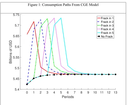
into the dynamic programming model. Figure 1 illustrates the consumption paths with spikes
occurring at the time of fracking. After the initial shock, fracking stops as reserves are depleted
and consumption falls, reaching a new steady state. To test for sensitivity to the price of oil and
gas, the CGE model is used to evaluate the impact of fracking bans over a range of prices. Oil
and gas prices are assumed to move together, increasing and decreasing from base values in
equal proportions. Given our base specification, the annuitized value of the consumption benefits
22
Figure 1: Consumption Paths From CGE Model
Note: The x-axis is the policy period, which are five-year increments. The y-axis is consumption in billions of dollars. All simulations include normal growth shocks in year 1.
4.2 Parameterization of Damages
In order to solve the model, we also parameterize the initial beliefs about the distribution of the
monetary value of fracking damages,η. Given additive separability, this can occur
independently from the parameterization of economic benefits described above. Recall that η is
normally distributed with initial beliefs about the mean and standard error equal to µ0 and σ0 2
,
respectively. The magnitude of these damages must be weighed against the consumption
benefits of fracking, calculated in section 4.1.
To parameterize current beliefs about this distribution, we define a plausible range within which
0 1 2 3 4 5 6 7 8 9 10 11 12 13
Periods
5.4 5.45 5.5 5.55 5.6 5.65 5.7 5.75
Billions of USD
23
the monetary value of damages is likely to fall. First, we assume a 5% chance of negative
damages (i.e., benefits) from fracking. This could occur if, for example, fracking allows natural
gas to displace coal in local energy production, leading to cleaner air. At the other extreme, we
assume that damages could exceed a high-damage scenario with a probability of 5%.
To define the high-damage scenario, we calculate the monetary cost of purchasing water rights to
permanently replace the current surface water supply18. We assume the municipality would
obtain shares in the Colorado-Big Thompson (C-BT) System, where water rights have sold for
$50,000 per acre-foot (http://bizwest.com/water-prices-reach-historic-highs/). To calculate the
number of shares that the municipality would need to purchase, we use the Colorado City of Fort
Collins’ water use as an example. If Fort Collins Utilities had to purchase C-BT shares to cover
100% of its population of 150,000, it would need to purchase 51,805 acre-feet19. Assuming the
representative municipality of 50,000 people would use the same initial mix of C-BT and
non-C-BT water sources and consumption per capita as Fort Collins, it would need to purchase 17,268
acre-feet from C-BT (valued at $50,000 per acre-foot) for a total one-time cost of $863 million.
Amortized over 10 (5-year) periods with a discount rate of 5%, this high-damage estimate
becomes approximately $200 million per period.
The 5% upper ($200 million) and lower ($0) tails of fracking damages allow us to calculate the
mean and standard error of the distribution. Figure 2 displays the distribution of fracking
18
Although surface water moves very rapidly, on the order of meters per second, the pollutants can linger for decades if they are highly recalcitrant, like organochlorines or polychlorinated biphenyls (Baumann and Whittle 1988; Hooper et. al 1990; Garton et. al 1996) or radioactive (radon is naturally occurring in the uranium-rich soil of Colorado).
24
damages given the specified two tails. From Figure 2, we can see that the mean of the per-period
fracking damages is ~$100 million per period. The standard deviation of this distribution is $60
[image:25.612.129.487.176.516.2]million. Therefore, our initial beliefs are µ0=$100 million and σ0 =$60 million. .
Figure 2: Distribution of Environmental Damages Given Calibrated Initial Beliefs
Note: The x-axis is the value of the damage parameter, in millions of dollars. The y-axis is the probability. The 5% tails are shaded.
If fracking is allowed, fracking damages will be realized and, from the perspective of the
policymaker, drawn from this distribution. If, on the other hand, fracking is banned, a
policymaker anticipates receiving a signal that will provide information about the distribution of
25
Recall that the annuitized present value of the consumption benefits of fracking today is
approximately $113.6 million per period. This suggests that, in expectation, the net benefits of
fracking are positive. Under a naïve net-present value rule, a risk neutral policymaker would
therefore allow fracking because the expected benefits exceed the expected costs. Nevertheless,
a policymaker that anticipates learning about the distribution of damages will wait before
allowing fracking if the QOV is sufficiently valuable. To find the conditions under which a
policymaker would continue to ban fracking we solve the parameterized dynamic option value
model using the rule described in Equation 4.
5. Results
We first solve the model for a range of initial beliefs about damages and a range of assumptions
about the rate of learning and examine if the ability to learn influences the optimal policy
decisions. Then, we compare the role of learning to other factors such as the value of oil and gas
reserves. Next, we quantify a monetary value of the QOV and use Monte Carlo simulations to
show that faster learning leads to better decision-making over time. We finish with tests for the
robustness of the results.
5.1. Optimal policy
To explore the impact of learning on the optimal policy decision, we solve the model for a range
of values for the standard error of the signal noise, presented in Equation 1. Specifically, we are
interested in estimating Equation 4 which compares theNPV
t (the present value of the expected
net increase in utility units from fracking) with estimates of QOVt(quasi-option value) and SOVt
(simple option value). If the NPV is greater (less) than the sum of QOV and SOV, then it is
26
Using the results from the CGE model discussed above and the estimates for QOV and SOV,
Figure 3 presents the optimal initial-period policy for fast (σε=$1), medium (σε= $200
million), and slow (σε =$500 million) rates of learning as a function of initial beliefs about
environmental damages. We also display the no-learning case. These curves mark the initial
belief combinations where the policymaker is indifferent between allowing fracking and
maintaining the ban. Intuitively, as learning becomes faster, there are fewer combinations of
initial beliefs (less area under the curve) for which fracking is optimal. The parameterized initial
beliefs are labeled and it becomes clear that the optimal policy in the calibrated model is
sensitive to the rate of learning. When learning is slow, the optimal policy is to allow fracking
since new information is relatively uninformative and unlikely to change next period’s policy. In
this case, the expected gains from fracking dominate the value of learning in influencing the
optimal policy. Under the parameterized beliefs, it is optimal to maintain a ban, receive precise
information about fracking damages, and revisit the decision next period if learning is fast. The
ban occurs despite positive expected net benefits from fracking, so a simplistic benefit-cost
framework that does not anticipate learning—a now or never approach—would allow fracking.
When σε =$211 million, the risk averse policymaker is indifferent between fracking and
banning given the parameterized initial beliefs. This implies that the policymaker should
implement a ban if she anticipates at least a 7.5% reduction in 𝜎!! over the first 5 years (1 model
period).
Notice that all three policy boundary curves converge to the same mean, µ0=$111.8 million as
σ0→0. This occurs because information is only valuable under uncertainty. We denote this
27
that µ0<µˆ with low initial uncertainty (southwest corner) will result in a FRACK policy.
Similarly, beliefs that µ0 >µˆ and the initial uncertainty is high (northeast corner) will result in a
BAN policy. Increasing uncertainty while holding µ0=µˆ makes a ban more likely, due to the
ability to learn about the true distribution. Even with no learning, risk aversion means that higher
uncertainty can push towards a BAN.
5.2. Learning and the Value of Energy Resources
Figure 3 reveals that learning can play a pivotal role in the policy decision holding other
economic factors constant. Now, we compare the impact of improved learning to changes in the
[image:28.612.123.492.242.515.2]resource value. We use the CGE model to compute the benefits of fracking for four oil and gas Figure 3: First Period Optimal Policy
Note: The x-axis is the initial mean damage belief. The y-axis is the initial standard error belief. Each curve demarks where policy switches. Fast learning is 𝜎! =$1, medium learning is 𝜎! =$200 million, and slow learning is 𝜎!=$500 million; and the initial
beliefs used in the calibration exercise are 𝜇!,𝜎! =(100,60) million dollars. The slope
28
prices. Then, we fit a benefit function, b t
(
,f,p)
, that maps current time period (t), whenfracking began (f), and price of oil (p) into a dollar value of consumption benefits, (C):
b:
(
t,f,p)
→C. With this, we populate a consumption benefit matrix for a range of oil pricesfrom $30 to $90 per barrel in $5 intervals and solve for both the value of learning and the value
of fracking using Equation 5. The results are presented in Figure 4. The speed of learning is
expressed as the number of signals required to reduce the standard error by half of its initial
level. The figure highlights the policymaker’s willingness to trade off faster learning for
decreased economic benefits through a lower reserve value. We display the policy boundary
curve with calibrated beliefs as well as for higher and lower initial standard errors for the
damages distribution.
Figure 4 shows that improvements in the rate of learning can tilt the decision towards a
temporary ban, but that the price of oil – and the value of reserves – has a substantial influence
on the decision. Improving the rate of learning only affects the first period decision in a small
range of prices. This is true even in the high-initial variance case (dotted line Figure 4). On the
other hand, a price change from $45 to $55 per barrel likely changes optimal policy in this
context. In our parameterized scenario (solid black line with dot markers in Figure 4), a five
period reduction in the number of periods required for the variance belief to reduce by half is
equivalent to an increase in oil price from $41.92 to $47.88 per barrel – around a $6 change.
For comparison, between August 2015 and August 2016, oil prices ranged from ~$30 per barrel
to nearly $55. This suggests that changes in price expectations consistent with existing oil price
volatility could have a much larger impact on decision-making than improvements in the speed
29
value of reserves, which, in turn, is influenced by the size of the reserve, the price of oil and gas,
and local mineral rights ownership. Our calibrated example shows that the ability to learn can
[image:30.612.105.511.169.470.2]play a pivotal role, provided the value of reserves falls within a relatively narrow range20.
Figure 4: First Period Optimal Policies for 3 Different Initial Beliefs
Note: The x-axis represents the speed of learning as the number of signals for 𝜎!= .5𝜎! where a
time period is 5 years. The y-axis is the price of oil in dollars per barrel. The 3 curves are a mean-preserving spread. The slopes are the willingness to avoid a slower rate of learning in terms of reduced net benefits.
5.3 Quantifying the Option Value
Despite the relative importance of the value of reserves, the calibrated economy-wide QOV
remains large, even in comparison to the consumption benefits of fracking. In order to calculate a
monetary value of the QOV, we solve the model under risk neutrality. This enables us to express
20
This also suggests that the option value associated with learning about the price of oil may be quite large compared to learning about damages. This should be explored in future work.
0 1 2 3 4 5
Periods until
σ
2t
is 50% of
σ
2 0 3035 40 45 50 55 60
Price of Oil ($/barrel)
(µ0,σ 0) = (100,40) (µ0,σ
0) = (100,60) (µ0,σ
0) = (100,80)
30
all value functions and option values in monetary units. Since the monetary value of the QOV
increases with risk aversion it is likely these results represent a lower bound for the impact of
[image:31.612.99.518.171.493.2]learning on policy decisions.
FIGURE 5: Value Functions and QOV under Risk Neutrality
Note: The x-axis is the standard error of the noisy signal. The y-axis is the monetary value in millions of dollars. As learning becomes slower, the QOV decreases pulling the full value of sophistication, which approaches the SOV asymptotically. The maximum value of the QOV occurs where 𝜎!→0 and is 61.1 million dollars.
Figure 5 shows how the numerical value of the first-period QOV depends on the standard error
of the signal (σε). Recall that the QOV is the difference between the Vsoph and the simple option
value (Equation 6). All three reflect present values denominated in initial-period monetary units.
The QOV is largest ($101.5 million - $40.4 million = $61.1 million) when σε is smallest
31
calibrated setting when 𝜎! =$177 million (labeled in Figure 5). At this learning rate, the initial
variance drops 10% after the first signal. Recall that the cutoff under risk aversion (ρ=2) in
Figure 3 was σε =$211 million, showing that a risk neutral policymaker requires faster learning
(all else equal) to justify a fracking ban.
These QOV represents the value of information acquired during a temporary ban and its
numerical value indicates that it is an economically important social value. When learning is fast,
the QOV represents 12.76% of the $478.99 million in gross consumption benefits that fracking
brings (in present value terms). To our knowledge, this is the first attempt to quantify a
numerical, economy-wide QOV associated with an environmental policy decision.
5.4. Policy Simulation
Thus far, our results indicate that faster learning increases the QOV, incentivizing a moratorium
on fracking, in the initial period. However, this does not show that policymakers interested in
supporting economic development activities should prefer slow learning. Instead, as is intuitive,
faster learning leads to better decision-making over time, both increasing fracking instances
when it is beneficial and decreasing instances when it is not. To illustrate this, we simulate policy
decisions for the base model (ρ=2) over a range of η*, from $60 million to $180 million (i.e.,
spanning the calibrated µˆso that when η*is greater (less) than µˆbanning (fracking) is optimal ex
post). The signals (described in Equation 1) depend on η*even when initial beliefs are held
constant. We consider the fast and medium learning rates defined in section 5.1 and presented in
Figure 3. This means that the first period decision is always BAN (H1=0) For each learning
rate, σε, and then for each η*, we draw 1000, four-element, signal sequences, s t
{ }
t=1t=4
32
distribution η*
,σ0
2 +σε
2
(
)
. The calibrated beliefs (100, 60), in millions of dollars, are the initialdamage beliefs (µ0,σ0 2
), which evolve over time according to Equations 2a and 2b, depending
on the random signal sequence. We evaluate and compareVtsoph Ht−1,µt,σt2
(
)
andNPVt Ht
−1,µt,σt 2
(
)
for t=2, 3, 4, 5 to find the optimal policy in accordance with Equation 4.The results of the simulations are presented in Figure 6. Results are displayed as the probability
of making the correct (or incorrect) decision by the end of the 5-period decision horizon. In the
left panel, damages are less than the benefits so fracking is beneficial. Under fast learning,
fracking occurs 94% of the time by period 2 while with medium learning, it takes all 5 periods
before at least 79% of simulations result in beneficial fracking. Note that 97% of the fast learning
simulations frack by period 5, the terminal decision period. Recall that the policy switches at
𝜇= $111.8 million but the annualized consumption benefits are $113.6 million. The reason that
3% of the fast-learning simulations do not frack when it is beneficial is risk aversion. That is,
regardless of the level of certainty, a risk averse policymaker with mean beliefs
µt ∈
(
$111.8, $113.6)
, t=1, 2, 3, 4will ban fracking under uncertainty even though it would bringan increase in net welfare ex post.
The right panel presents the result of simulations in which damages exceed the benefits, so a
fracking ban optimizes ex post welfare. In this case, under fast learning an initial ban results in
the optimal decision in every instance (i.e., the probability of fracking is always zero). On the
other hand, under medium learning, there is a 45% chance fracking will eventually be allowed,
33
Figure 6 illustrates that, despite incentivizing a moratorium in the first period, faster learning
[image:34.612.80.535.145.452.2]results in more fracking when it is beneficial and less when it is not.
Figure 6: Simulation Results: Probability of Fracking in or before each Period
Note: The x-axis is the time period in which fracking begins. Each time period represents 5 years. The y-axis is the percentage of simulations in which fracking occurs in time, 𝑡. The left panel is the simulations for which 𝜂∗is less than the present value of consumption benefits. The right panel is the simulations for which 𝜂∗
exceeds the present value of consumption benefits In comparison to medium learning (𝜎!=$200 million),
faster learning (𝜎! = $1) results in more fracking and sooner when it’s beneficial and no fracking when it is
not.
5.5. Sensitivity analyses
In Figure 7, we explore the sensitivity of our conclusions to assumptions about initial damage
distributions and risk aversion. First, we test robustness of the results to changes in initial beliefs.
The results in Figure 4 present the policy boundary curves under a mean-preserving spread of the
34
left panel of Figure 7 shows that the main conclusions are robust to these changes. Conditional
on the initial beliefs, increasing the rate of learning has a relatively small impact on the policy
decision. Initial beliefs about the mean do have a notable impact on the (still narrow) price range
within which increasing the rate of learning plays a pivotal role in determining optimal policy.
In the right panel of Figure 7, we assess the impact of changing the coefficient of relative risk
aversion. The panel replicates the base curve in Figure 4 using a range of values for 𝜌. As
expected, increasing 𝜌 raises the oil prices for which a ban is optimal. It also increases the
importance of the rate of learning in influencing the policy decision, indicated by the steeper
slope of the high risk aversion boundary curve in Figure 7. Despite this, even at high levels of
[image:35.612.106.508.382.672.2]risk aversion,the range of prices where learning is influential remains narrow.
Figure 7: Model Sensitivity
35
6. Discussion and Conclusion
Uncertainty about fracking damages and the ability to learn create a QOV that can impact the
economic rationale for imposing a temporary ban on fracking activities. In our calibrated setting,
we show that a moratorium can be justified if beliefs about environmental damage variance are
expected to drop at least 7.5% before the decision is revisited (or 10% for a risk neutral
policymaker). Faster learning also leads to better decision-making over time. Though learning
can influence optimal policy, we find that its role is relatively unimportant when compared to
plausible (indeed historical) fluctuations in the price of oil.
Although we emphasize a model of fracking policy, the developed methodology expands the
class of problems that can be quantitatively approached with an option value framework.
Juxtaposing a detailed CGE model with a dynamic learning framework makes it possible to
quantify the impact of uncertainty and learning within an empirically grounded general
equilibrium setting. The approach could be useful in other policy contexts, including public
infrastructure investment or public safety measures.
In addition to the policy-relevant observations above, several other policy implications can be
drawn from the analysis. First, uncertainty may push local policymakers to temporarily ban
fracking until better information about associated damages becomes available. Consider the 2005
Energy Policy Act, which amended the 1974 Safe Drinking Water Act to exclude fracking
injection fluids (other than diesel fuels) from the EPA’s oversight, while exempting extraction
companies from disclosing the chemicals involved in fracking operations. This served to increase
public uncertainty about the dangers of fracking which makes adopting a ban more attractive
36
Next, the rate of learning influences local policy decisions in a context of uncertain fracking
damages. A high rate of learning makes a first period ban more appealing but makes fracking, if
beneficial, more likely in subsequent periods. The value function when the decision remains
(Equation 3) is weakly increasing in the rate of learning, implying that faster learning cannot
decrease welfare. Consequently, the public has an interest in reducing the noisiness around
fracking information through, for example, research and improved industry transparency.
Although the potential for learning could push a community to implement a temporary ban, it
also creates the incentive to remove the ban if this is in their interest. Many policy options exist
to support the opportunity for learning. These include funding for scientific research on impacts,
information provision that enables homeowners to better negotiate with oil and gas companies
(see Timmins and Vissing 2014), encouraging municipalities to fund their own studies21, and
providing assistance with local impact studies.
Our quantification of the QOV highlights an intriguing dimension of local fracking policy. The
information-revealing signal about fracking damages is a public good. The ability to ban fracking
and learn from others’ experiences in similar, perhaps nearby, regions implies a free-rider
problem where local jurisdictions obtain the benefits of information without contributing to its
production. The full value of sophistication represents the local jurisdiction’s willingness to pay
for the ability to ban fracking and learn but there are currently no institutions that allow for its
capitalization.
While useful, the model presented here has some important limitations. First, we assume that
fracking policy is a binary (yes/no) decision. Feasibly, policymakers could choose both when to
21
After the 2013 moratorium, The City of Fort Collins hired a consulting firm to study the direct impacts of fracking. The report was able to provide dollar ranges of health and property damages:
37
frack and at what intensity. When decisions are adaptable over time, the ability to learn tends to
increase the level of development in early periods (Karp and Zhang 2006). Allowing a small
amount of fracking in certain areas of a given jurisdiction could result in very precise
information about the true value of damages. Then, policymakers could adjust the amount of
fracking to ensure optimality. This is similar to the result in Karp and Zhang (2006) that the
ability to learn about climate sensitivity can increase early emissions levels. Despite this, binary
policies such as local bans are common in practice and likely reflect political or legal constraints
that prevent policymakers from employing more delicate instruments. Indeed, many bans have
arisen through the blunt instrument of local referenda.
Second, we ignore the stochastic nature of energy prices. In reality, policymakers also learn
about the value of the reserves they control. If prices have an upward drift, for example, this
would create a further incentive to wait before fracking is allowed and oil and gas reserves are
exploited. Future work should consider the interaction between stochastic energy prices and
uncertain environmental damages.
Another limitation is that consumption benefits do not capture distributional effects. It could be
that the economic benefits accrue to a small fraction of the local population. Routine burdens,
including noise and light pollution or increased traffic, tend to affect those most closely located
to fracking operations (Gopalakrishnan and Klaiber 2014), but as Hill (2013) points out these are
often socio-economically disadvantaged groups that may not receive the benefits from fracking.
A mismatch between those that benefit and those that incur the costs from fracking is not
considered here but future work should investigate how this could affect the local political
38
Despite the limitations of the model developed here, it provides a useful tool for evaluating the
economy-wide net benefits of oil and gas development for a range of economies, from local to
national scales. A numerical QOV model has the potential to explain existing decisions or to
inform policy choices in the future. Our results suggest that when the net benefits of fracking,
including consumption benefits and environmental damages, are not clear, the ability to learn
about uncertain fracking damages over time can play a pivotal role in the decision-making
process. This was revealed in our calibrated example but this lesson can be applied more
39
REFERENCES:
Aguilera, Inmaculada, Guxens, M., Garcia-Esteban, R., Corbella, T., Nieuwenhuijsen, M. J., Foradada, C. M., & Sunyer, J. "Association between GIS-based exposure to urban air pollution during pregnancy and birth weight in the INMA Sabadell Cohort." Environmental health perspectives 117.8 (2009): 1322.
Allcott, Hunt, and Daniel Keniston. Dutch disease or agglomeration? The local economic effects of natural resource booms in modern America. No. w20508. National Bureau of Economic Research (2014).
Arrow, Kenneth J., and Anthony C. Fisher. "Environmental preservation, uncertainty, and irreversibility." The Quarterly Journal of Economics (1974): 312-319.
Bennett, Ashley, and John Loomis. "Are Housing Prices Pulled Down or Pushed Up by Fracked Oil and Gas Wells? A Hedonic Price Analysis of Housing Values in Weld County, Colorado." Society & Natural Resources (2015): 1-19.
Bond, Craig A., and John B. Loomis. "Using numerical dynamic programming to compare passive and active learning in the adaptive management of nutrients in shallow lakes." Canadian Journal of Agricultural Economics/Revue canadienne d'agroeconomie 57.4 (2009): 555-573