Munich Personal RePEc Archive
Estimation and Inference of Threshold
Regression Models with Measurement
Errors
Chong, Terence Tai Leung and Chen, Haiqiang and Wong,
Tsz Nga and Yan, Isabel K.
The Chinese University of Hong Kong, Xiamen University, Bank of
Canada, City University of Kong Kong
5 November 2015
Online at
https://mpra.ub.uni-muenchen.de/68457/
Estimation and Inference of Threshold Regression
Models with Measurement Errors
Terence Tai-Leung Chong
∗, Haiqiang Chen
†, Tsz-Nga Wong
‡and Isabel Kit-Ming Yan
§5/11/2015
Abstract
An important assumption underlying standard threshold regression models and their variants in the extant literature is that the threshold variable is perfectly measured. Such an assumption is crucial for consistent estimation of model parameters. This paper provides the first theoretical framework for the estimation and inference of threshold regression models with measurement errors. A new estimation method that reduces the bias of the coefficient estimates and a Hausman-type test to detect the presence of measurement errors are proposed. Monte Carlo evidence is provided and an empirical application is given.
Keywords: Threshold Model; Measurement Error; Hausman-type Test.
JEL Classification: C12, C22.
∗Corresponding author, Terence Tai-Leung Chong, Institute of Global Economics and Finance and
Depart-ment of Economics, The Chinese University of Hong Kong, Hong Kong and DepartDepart-ment of International Eco-nomics and Trade, Nanjing University, China. E-mail: [email protected]. We would like to thank Leonard Stefanski, W.K. Li, George Kapetanios and seminar participants at City University of Hong Kong, Lingnan Uni-versity and International Symposium on Econometric Theory and Applications (SETA) for helpful comments. We also thank Min Chen and Margaret Loo for their able research assistance. All remaining errors are ours.
†Wang Yanan Institute for Studies in Economics, Xiamen University; E-mail: [email protected]. ‡Bank of Canada
1
Introduction
Measurement error is a common problem in economic data. In particular, macroeconomic data on consumption, unemployment, inflation, and variables that are intrinsically unobservable are often subject to measurement errors because of data aggregation or for other reasons. Madan-sky (1959) shows that the presence of measurement errors results in inconsistent estimation of parameters in a linear model. Amemiya (1985, 1990) and Schennach (2004) investigate the measurement error problem in nonlinear models. A recent study by Xia and Tong (2011) pro-poses a method based on feature matching to estimate time series models with measurement errors. The aforementioned methods focus on measurement errors in the explanatory variables, however. Thus far, no study in the literature has attempted to explore the problem of measure-ment error in the context of threshold regression models. In the presence of measuremeasure-ment errors in the threshold variable, the observations cannot be correctly ranked according to their true values, which can render the estimator inconsistent in such models. This paper provides the
first theoretical framework for the inference and estimation of a threshold regression model with measurement errors. Empirically, there is an important distinction between measurement errors in explanatory variables and measurement errors in the threshold variable. In the former case, where the measurement error is often assumed i.i.d. additive to the regressors, all observations of the regressors are confounded by the measurement error. As a result, the true model parame-ters cannot be retrieved from any subsets of the observations. In the latter case, however, the existence of measurement errors may not lead to misclassification of observations.1Therefore, one
can improve the parameter estimates of a threshold regression model by estimating a subsample where misclassification is unlikely to occur.
The contribution of our paper is twofold. First, we propose a new method that reduces the bias of the parameter estimates in the presence of measurement errors. Second, we develop a Hausman-type test (Hausman, 1978, 2001; Jeong and Maddala, 1991) for measurement errors in the threshold variables. We apply our test to reestimate the growth convergence model of Hansen (2000), using the per capita output and adult literacy rate as threshold variables. Since the data are taken from earlier years, these two variables might suffer from measurement error. Our test results suggest the existence of measurement errors in both threshold variables. We re-estimate the model andfind that the convergence hypothesis only holds for countries with lower initial per capita output or those with higher adult literacy rate, which differs from Hansen’s (2000) results.
The rest of the paper is organized as follows. Section 2 presents the theoretical model and the
1For instance, consider the case where the threshold variable is the GDP per capita. It is unlikely that a
underlying assumptions. Section 3 proposes a new method to reduce the bias of the parameter estimates. A new test for measurement errors is developed in Section 4. Section 5 provides Monte Carlo evidence for our theory. An empirical application is presented in Section 6 and Section 7 concludes the paper. All proofs are relegated to the appendix.
2
The Model
Threshold regression models have developed rapidly since the seminal work of Tong and Lim (1980), and Tong (1983): for example, the smooth transition threshold model (STAR) of Chan and Tong (1986); the functional-coefficient autoregressive (FAR) model of Chen and Tsay (1993); the threshold autoregressive heteroscedastic model of Li and Lam (1995) and Li and Li (1996); and the nested threshold autoregressive (NeTAR) model of Astatkie, Watts and Watt (1997), among others. The model was further extended to allow for multiple threshold values in Tsay (1998) and Gonzalo and Pitarakis (2002). More recently, Chen et al. (2012) investigated the statistical properties of threshold estimators in regression models with multiple threshold vari-ables.2 Hansen (2011) and Tong (2011) review the development of the threshold model in time
series analysis since the 1980s.
The aforementioned studies, however, assume that the threshold variable is not error-ridden. If the threshold variable is measured with errors, some observations could be misclassified, and the parameter estimates will be inconsistent. Consider the following threshold regression model:3
=1+ (2−1)Ψ0 (0) + (1)
where and denote the dependent variable and the regressors respectively. 1 and2 are the
pre-shift and post-shift regression slope parameters respectively. Ψ0
(0)is an indicator function,
which equals one when the true threshold variable0
exceeds the threshold 0. That is,
Ψ0 (0) =¡0 0¢ (2)
In the presence of measurement errors, the true value of the threshold variable cannot be ob-served.4 Instead, we observe
=0+
2The threshold effect is also considered in modelling conditional distributions (see Wong and Li, 2010). 3We consider a univariate model for illustration purposes. The extension to multivariate
is provided in the
appendix.
4If regressors are also measured with errors, we can use the projection theorem to rewrite the model as a
where represents the observed threshold variable which is contaminated with measurement
errors. Let Ψ()be the observed indicator function defined based on the observed threshold
variable
Ψ() =( ) =
¡
0 −
¢
=Ψ0 (−) (3)
Using the observed data { }=1, the above threshold model can be estimated by the
following profile least squares (LS) estimation method.5 The threshold value
0 is estimated by
minimizing the sum of squared residuals:
b
= arg min
∈Γ () (4)
where
() =
X
=1
³
−b1()−(b2()−b1())Ψ()
´2
(5)
Given the threshold estimateb the estimators for1 and2 are respectively
b
1(b) =
X
=1
(1−Ψ(b))
Ã
X
=1
2 (1−Ψ(b))
!−1
(6)
and
b
2(b) =
X
=1
Ψ(b)
Ã
X
=1
2Ψ(b)
!−1
(7)
Before proceeding further, we impose the following assumptions on the threshold model and the measurement error.
1 : is strictly stationary, ergodic and − with − coefficients satisfying
P∞
=1 12
∞.
2 : is a martingale difference sequence and (|z−1 0) = 0 wherez−1 is the past
information set of{ };6 and sup||2+ ∞ for some 0.
3 : (||4)∞ and (||4)∞
4 : 0
is strictly stationary and has a continuous distribution (). Let () denote the
density function satisfying ()≤ ∞ for all ∈Γ and (0)0
5 : is i.i.d. random variable with zero mean and constant variance 2. is independent
of { 0 }
6 : =2−1 = 06 and0 ∈Γ= [ ]
5The estimation method for threshold model is similar to that of structural-change models (Hansen, 2000 and
Chong, 2001).
6For cross-sectional data, the past information setz
A1 to A4 are standard assumptions in the literature on threshold models. Assumption 5
assumes the measurement errors to be independent of the regressors and the threshold variable. This assumption is imposed to simplify the proof. One might relax this assumption slightly to allow for the mis-measured threshold variable to be one of the regressors. Section 5 of this paper also reports the results for the self-exciting threshold autoregressive model (SETAR), where both and are the lags of . Assumption 6 assumes the presence of the threshold effect and
that the true threshold value0 falls into a proper subset of the threshold variable space.
Lemma 1: Under Assumptions 1−6, we have
b
1(b)−1 =
P
=12 [Ψ(0+)−Ψ(max{0+b})]
P
=12 (1−Ψ(b))
+( 1 √
) (8)
and
b
2(b)−2 =−
P
=12 [Ψ(b)−Ψ(max{0+b})]
P
=12Ψ(b)
+( 1 √
) (9)
Lemma 1 shows that the two conventional LS based estimators b1(b) and b2(b) are in-consistent in the presence of measurement errors even at b = 0. Note that Ψ(0 +) −
Ψ(max{0+b}) = ( (0+)) − ( max{0 +b}) is always non-negative.
Thus, when 0, b1(b) will be biased upward and b2(b) will be biased downward, and vice versa.
3
The New Estimator
In this section, we propose a method that reduces the bias of the estimates of 1 and 2. For afixed ∈(012) definee1() ande2() as the pre- and post-shift OLS estimators using the
lowest [] ordered observations and the highest [] ordered observations in a sample with observations. Denote and as the empirical lower and upper -quantiles of the threshold variableWe have
e
1() =
X
=1
³
1−Ψ
³
´´
Ã
X
=1
2 ³1−Ψ
³
´´
!−1
(10)
e
2() =
X
=1
Ψ()
Ã
X
=1
2Ψ()
!−1
Note that e1()and e2() can be considered as weighted OLS estimators of 1 and2
respec-tively with zero weight given to the middle range.
Lemma 2: Under Assumptions 1−6,we have
e
1()−1 =
P =12
h
Ψ(0+)−Ψ
³
maxn0+
o´i
P =12
³
1−Ψ
³
´´ +(
1 √
) (12)
and
e
2()−2 =−
P
=12 [Ψ(P)−Ψ(max{0+ })]
=12Ψ()
+( 1 √
) (13)
Lemma 2 shows that the estimators e1() and e2() are inconsistent in the presence of measurement error. The bias term is related to the distribution of the measurement error
and the cutting values and 7 The following theorem shows that the new estimators have
smaller bias than conventional LS estimators given the existence of measurement errors.
Theorem 1: Under Assumptions A1 to A6, for any b ∈ (, ), e1() and e2() are less
biased thanb1(b) andb2(b) when2
0.
Note that Theorem 1 is established under the condition thatb ∈( )This assumption is automatically satisfied if we defineΓ= (,)in Equation (6). In the literature,is commonly set at15% to ensure enough observations in the extreme regimes.
Note also that in the absence of measurement error, i.e.,2
= 0, the bias terms in Equations
(10), (11), (14) and (15) are all zeros, implying that both the full-sample estimators b1(b) and
b
2(b) and the new estimators e1() ande2() are consistent. Since, however, e1()and e2()
only use the data from a subsample, they will be less efficient than b1(b) and b2(b). On the
other hand, if there is any measurement error,e1()ande2()will be less biased. Theoretically, given b ∈ (, ), it can be shown that b1(b) andb2(b) are the limits of e1() and e2() as → 05. A larger improves the efficiency of the estimate, but it will also increase the bias caused by the measurement error. As the problem of low efficiency may be as serious compared to a high bias, the new estimators should perform better than the traditional estimators in terms of mean square errors (MSE). In Section 5, we show that under different model settings, e1()
ande2()have a smaller MSE than b1(b)andb2(b) in most cases.
4
Test Statistic
In this section we develop a test for measurement errors. Consider the following null hypothesis of no measurement error:
0 : 2 = 0
1 : 2 0
Recall that2
refers to the variance of the measurement error term. Letb =−b1(b)− (b2(b)−b1(b))Ψ(b) and define the following sample moments:
c
1() =
P
=12( ≤)
c
2() =
P
=12( )
and
b
Ω11(1 2) =
P
=12( ≤1)b 2
( ≤2)
b
Ω12(1 2) =
P
=12( ≤1)b2( 2)
b
Ω22(1 2) =
P
=12( 1)b 2
( 2)
Using the above sample moments, we construct a Hausman-type test for measurement error in the threshold variable, defined as
() =
à b
1(b)−e1()
b
2(b)−e2()
!0
b Π−1
à b
1(b)−e1()
b
2(b)−e2()
!
(14)
where
b
Π= d
à √
(b1(b)−e1()) √
(b2(b)−e2())
!
=
à b Π11Πb12
b Π0
12Πb22
and
b
Π11 = c1()−1Ωb11( )c1()−1+c1(b)−1Ωb11(bb)c1(b)−1
−c1()−1Ωb11(b)c1(b)−1−c1(b)−1Ωb11(b )c1()−1
b
Π12 = c1()−1Ωb12( )c2()−1+c1(b)−1Ωb12(bb)c2(b)−1
−c1()−1Ωb12(b)c2(b)−1−c1(b)−1Ωb12(b )c2()−1
b
Π22 = c2()−1Ωb22( )c2()−1+c2(b)−1Ωb22(bb)c2(b)−1
−c2()−1Ωb22(b)c2(b)−1−c2(b)−1Ωb22(b )c2()−1
The following theorem establishes the null asymptotic distribution for the test statistic.
Theorem 2: Under Assumptions A1 to A6, for 0 ∈ (, ) we have () ⇒ 22 under
0 :2 = 0
This result can easily be extended to models with regressors, where the corresponding degree of freedom is 2. The asymptotic null distribution is not affected by the choice of under the null hypothesis if the condition 0 ∈ (, ) is satisfied. The value of however, might affect the precision of the parameter estimates and the power of the test infinite samples. In the following simulations, we consider different 0 to examine their impact on estimation
and testing. Note that, under the alternative hypothesis, b1(b)−e1() andb2(b)−e2() are
(1)and () diverges to infinity. Therefore, the test is consistent.
5
Monte Carlo Simulations
Experiment 1: Estimation performance of the new estimators
To demonstrate that the use of the restricted sample (the sample excluding the middle100 (1−2)% of the ordered observations) can reduce the estimation bias, we examine thefinite sample per-formance of the new estimator.8 We consider the following four data generating processes:
DGP 1: Mean-shift model
=1(0 ≤0) +2
¡
0 0¢+ = 12 (15)
DGP 2: Univariate threshold regression model with conditional heteroskedasticity
=1(0 ≤0) +2
¡
0 0
¢
+ (02) = 12 (16)
DGP 3: Threshold autoregressive model (TAR)
= (11−1+12−2)(0 ≤0) + (21−1+22−2)
¡
0 0
¢
+ = 12 (17)
DGP 4: Threshold regression model where the threshold variable is one of the regressors
= (11+120)(0 ≤0) + (21+220)
¡
0 0¢+ = 12 (18)
The observed threshold variable is specified as =0+ where 0 ∼ (101) and
the measurement error ∼. (0 2) follows an (010) distribution. ∼.
(01). 0 and are independent of each other. Let0 = 10 1 = 1 2 = 2 11 = 05
12 = 01, 21=−05 and22=−01
Note that for DGP 4, in the estimated model, the second regressor is which is affected by
the measurement error. Thus, it violates Assumption 5.
For all cases, we replicate the simulations with = 1000400 or 200 (sample size) and = 1000 (number of replications).
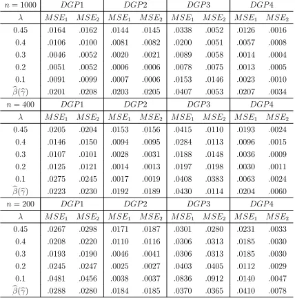
Table 1 reports the mean squared errors (MSE) of the estimators. For each sample size, we study the cases for = 0102 03 04 and 045. The MSE of e1() and e2() are reported in the first four rows of each panel, and the last row reports the MSE of the conventional LS estimatorsb1(b)andb2(b)from the full sample.9 The simulation shows that, for most cases, as
the sample size increases,e1()ande2()have smaller MSE than the conventional LS estimators
b
1(b) andb2(b)in the presence of measurement errors, which is consistent with Theorem 1.10
Table 1: Performance of the estimators (2
= 025)
9For DGP3 and DGP4, 1= (b11) + (21b )and 2= (b12) + (b22)
10In empirical studies, an important question is tofind the optimal value forA possible solution is to use the
= 1000 1 2 3 4
1 2 1 2 1 2 1 2
045 0164 0162 0144 0145 0338 0052 0126 0016 04 0106 0100 0081 0082 0200 0051 0057 0008 03 0046 0052 0020 0021 0089 0058 0014 0004 02 0051 0052 0006 0006 0078 0075 0013 0005 01 0091 0099 0007 0006 0153 0146 0023 0010
b
(b) 0201 0208 0203 0205 0407 0053 0207 0034
= 400 1 2 3 4
1 2 1 2 1 2 1 2
045 0205 0204 0153 0156 0415 0110 0193 0024 04 0146 0150 0094 0095 0284 0113 0096 0015 03 0107 0101 0028 0031 0188 0148 0036 0009 02 0125 0121 0014 0013 0197 0198 0030 0011 01 0275 0245 0017 0019 0408 0383 0063 0024
b
(b) 0223 0230 0192 0189 0430 0114 0204 0060
= 200 1 2 3 4
1 2 1 2 1 2 1 2
045 0267 0298 0171 0187 0301 0280 0231 0033 04 0208 0220 0110 0116 0306 0313 0185 0030 03 0193 0190 0046 0041 0306 0313 0185 0030 02 0245 0247 0025 0027 0403 0405 0112 0029 01 0481 0456 0038 0037 0836 0912 0140 0047
b
(b) 0288 0280 0184 0185 0370 0365 0410 0078
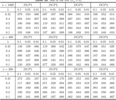
Experiment 2: The size and power of the test
[image:11.612.93.521.75.508.2]We study the size and power of the test statistic in this subsection. The data generating processes are the same with Experiment 1.
Table 2a reports the size of the test under the null of no measurement error for different DGP. When the sample size is large, the rejection rates are close to the asymptotic for all cases.
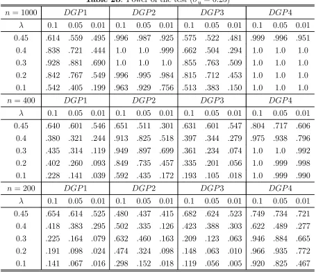
Table 2b reports the power of the test in the presence of measurement errors (2
= 025).
For DGP4, where the threshold variable is one of the regressors, the size remains unaffected, but the power is much improved. In this case, measurement errors exist in both the threshold variable and the regressor under the alternative hypothesis. This causes further bias of the estimates and may enlarge the value of the test statistic.
Table 2a: Size of the test (2
= 0)
= 1000 1 2 3 4
01 005 001 01 005 001 01 005 001 01 005 001 045 079 034 006 087 037 006 088 041 010 100 052 014 04 094 044 007 104 045 008 087 041 009 101 062 013 03 106 056 005 110 053 011 092 045 007 104 053 008 02 095 053 015 091 041 007 094 044 004 116 062 009 01 103 048 010 107 061 009 106 049 010 103 048 010
= 400 1 2 3 4
01 005 001 01 005 001 01 005 001 01 005 001 045 149 109 066 119 068 042 120 079 047 096 051 028 04 099 048 026 091 039 006 075 032 006 093 041 005 03 090 037 006 111 057 014 086 034 005 107 058 010 02 093 047 008 089 045 011 105 053 009 096 050 009 01 120 059 009 077 028 003 094 042 004 104 044 006
= 200 1 2 3 4
Table 2b: Power of the test (2
= 025)
= 1000 1 2 3 4
01 005 001 01 005 001 01 005 001 01 005 001 045 614 559 495 996 987 925 575 522 481 999 996 951 04 838 721 444 10 10 999 662 504 294 10 10 10 03 928 881 690 10 10 10 855 763 509 10 10 10 02 842 767 549 996 995 984 815 712 453 10 10 10 01 542 405 199 963 929 756 513 383 150 10 10 10
= 400 1 2 3 4
01 005 001 01 005 001 01 005 001 01 005 001 045 640 601 546 651 511 301 631 601 547 804 717 606 04 380 321 244 913 825 518 397 344 279 975 938 796 03 435 314 119 949 897 699 361 234 074 10 10 992 02 402 260 093 849 735 457 335 201 056 10 999 998 01 228 141 039 592 435 172 193 105 018 10 999 990
= 200 1 2 3 4
01 005 001 01 005 001 01 005 001 01 005 001 045 654 614 525 480 437 415 682 624 523 749 734 721 04 418 383 295 502 335 126 423 388 303 622 489 277 03 225 164 079 632 460 163 209 123 063 946 884 665 02 191 098 024 474 324 098 148 063 010 966 935 772 01 141 067 016 298 152 018 119 056 005 920 825 467
6
Empirical Application
Hansen (2000) examines the convergence hypothesis by analyzing the relationship between eco-nomic growth and the initial endowment of different countries. The baseline model is as follows:
85−60 =
⎧ ⎪ ⎪ ⎪ ⎪ ⎨ ⎪ ⎪ ⎪ ⎪ ⎩
1+1ln( )1960+1ln()+1ln(++) +1ln()+ if ≤
2+2ln( )1960+2ln()+2ln(++) +2ln()+ if
For country( ) denotes the real GDP per member of the population aged 15 to 64 in
year;85−60 = ln( )1985−ln( )1960 is defined as the difference of per capita real GDP
between 1960 and 1985; () refers to the average of investment to GDP ratio over the period
() is the average of the fraction of working-age population enrolled in secondary school
over the sample period. A negative value for in the regression provides evidence of convergence. We set+= 005, where is the growth rate of technology and is the depreciation rate. The threshold variables are the per capita output in 1960 and the adult literacy rate in 1960. We also allow for heteroskedasticity in the error term. Hansen (2000) provides estimation and testing results, assuming no measurement error in the threshold variable. The threshold value estimated for initial per capita is 863 with a 95% confidence interval [5941794], and the estimated threshold value for adult literacy is45% with a 95% confidence interval [19%57%]. The bootstrapping p-values of the Sup-LM test statistics for testing the presence of threshold effect are 0.088 and 0.214 respectively. Our point estimates for threshold values are very close to those obtained in Hansen (2000), where thefirst estimate is877 and the second is45%. The minor difference could be owed to the difference in the grid size.
In the model, the initial endowment is proxied by the per capita output, or the adult literacy rate measured in the 1960s. The use of proxies is likely to give rise to measurement errors, especially when the data are taken from early years. We apply the test developed in Section 4 with= 015to test for measurement error in per capita output and adult literacy rate. When the per capita output is used as a threshold variable, the test statistic value is4702 and the p-value is smaller than001. When the adult literacy rate is used as the threshold variable, the test statistic is 4569 and the p-value is smaller than 001. Therefore, we reject the null hypothesis of no measurement error in the threshold variable in both cases at the5%significance level.11
Tables 3a and 3b report the estimation results with per capita output and adult literacy rate as the threshold variables respectively. The first two columns report the results from the standard threshold model, and the last two columns report the results from the extreme regimes after the middle observations have been dropped. The heteroskedasticity-consistent standard errors are reported in parentheses.
11We also examine the test results by settingas 0102or03The null hypotheses are still rejected for all
Table 3a: Coefficient Estimations for Per Capita Output60
Traditional Method(b = 877) New Method (= 015)
60≤877 60877 60≤777 60 6527
431
(162)
∗ 366
(161)
∗ 477
(132)
∗ −149
(161)
ln( )1960 −065 (021)
∗ −032
(006)
∗ −079
(016)
∗ −0066
(016)
ln() 023
(0071)
∗ 049
(0144)
∗ 031
(0075)
∗ 047
(0082)
∗
ln(++) −029
(033) −(0025)49
∗ −043
(041) −(0115)43
∗
ln() 002
(0097) 0(03509)
∗ −003
(009) (00091)31
∗
Table 3b: Coefficient Estimations for Adult Literacy Rate60
Traditional Method (b = 4502) New Method (= 015)
60≤4502 604502 60≤15 6098
209
(187) (043196)
∗ 541
(233)
∗ 264
(203)
ln( )1960 −012
(016) −(0006)39
∗ −026
(025) −(0019)41
∗
ln() 017
(021) (008313)
∗ −011
(023) 0(02518)
ln(++) −039
(051) −(0027)42 (004339) −(0037)81
∗
ln() 045
(011)
∗ 0095
(013) (006611)
∗ 011
(014)
In Table 3a, the estimated coefficients forln()1960 are significantly negative in the model
using the full sample, which supports the convergence hypothesis. After the middle observations have been dropped, however, only the regime with lower per capita output supports the conver-gence hypothesis. The result is different from that of Hansen (2000). In Table 3b, our result shows that the convergence hypothesis holds only for countries with higher adult literacy rates, which corroborates Hansen’sfinding (2000).
7
Conclusion
[image:15.612.111.505.312.475.2]not lead to misclassification of observations, as the indicator variable for classifying observations may absorb some of the errors. If observations in the two extremes of the threshold spectrum have a lower probability of being misclassified, the estimates obtained from the full-sample will differ from those from a less contaminated subsample in the presence of measurement errors.
This paper develops a new test for the presence of measurement error in the threshold variable. Our test is based on the estimation difference between two estimators; thefirst assigns equal weight to each observation, and the second assigns zero weight to highly contaminated observations. Under the null hypothesis of no measurement error, both estimators are consistent, but the second estimator is less efficient. Under the alternative hypothesis, both estimators are inconsistent, but the second estimator is less biased. Our test statistic is shown to have an asymptotic Chi-square distribution. Monte Carlo evidence shows that the new test has good performance in terms of size and power. This paper also contributes to the literature by developing a new estimation method for reducing the bias of parameter estimates in the presence of measurement errors. Significant improvement in the parameter estimates is found by estimating a subsample with observations that are less likely to suffer from measurement errors. For future research in this line, one could extend our analysis to models with multiple regimes (Bai et al., 2008) and multiple threshold variables (Chen et al., 2012).
References
1. Amemiya, Y. (1985). Instrumental Variable Estimator for the Nonlinear Errors in Vari-ables Model. Journal of Econometrics 28(3), 273-289.
2. Amemiya, Y. (1990). Two Stage Instrumental Variable Estimators for the Nonlinear Errors-in-Variables Model. Journal of Econometrics 44(3), 311-332.
3. Armstrong, B. (1985). Measurement Error in Generalized Linear Models,Communications in Statistics: Simulation and Computation 14(3), 529-544.
4. Astatkie, T., D. G. Watts and W. E. Watt (1997). Nested Threshold Autoregressive (NeTAR) Models. International Journal of Forecasting 13(1), 105-116.
6. Chan, K. S. and H. Tong (1986). On Estimating Thresholds in Autoregressive Models.
Journal of Time Series Analysis 7(3), 179-190.
7. Chen, R. and S. Tsay (1993). Functional-Coefficient Autoregressive Models. Journal of the American Statistical Association 88, 298-308.
8. Chen, H., T. T. L. Chong and J. Bai (2012). Theory and Applications of TAR Model with Two Threshold Variables, Econometric Reviews 31(2), 142—170.
9. Chong, T. T. L. (2001). Structural Change in AR(1) Models. Econometric Theory 17(1), 87-155.
10. Chong, T. T. L. (2003). Generic Consistency of the Break-Point Estimator under Specifi -cation Errors. Econometrics Journal 6(1), 167-192.
11. Gonzalo, J. and J. Pitarakis (2002). Estimation and Model Selection Based Inference in Single and Multiple Threshold Models. Journal of Econometrics 110(2), 319-352.
12. Hansen, B. E. (2000). Sample Splitting and Threshold Estimation. Econometrica 68(3), 575-603.
13. Hansen, B.E. (2011). Threshold Autoregression in Economics. Statistics and Its Interface, 4, 123-127.
14. Hausman, J. A. (1978). Specification Tests in Econometrics. Econometrica 46(6), 1251-1271.
15. Hausman, J. A. (2001). Mismeasured Variables in Econometric Analysis: Problems from the Right and Problems from the Left. Journal of Economic Perspectives 15(4), 57-67.
16. Jeong, J. and G. S. Maddala (1991). Measurement Errors and Tests for Rationality.
Journal of Business and Economic Statistics 9(4), 431-439.
17. Madansky, A. (1959). The Fitting of Straight Lines when Both Variables are subject to Error. Journal of the American Statistical Association 54, 173-205.
18. Li, C. W. and W. K. Li (1996). On a Double-threshold Autoregressive Heteroscedastic Time Series Model. Journal of Applied Econometrics 11(3), 253-274.
20. Newey, W. K. and K. D. West (1987). A Simple, Positive Semi-definite, Heteroskedasticity and Autocorrelation Consistent Covariance Matrix. Econometrica 55(3), 703-708.
21. Schennach, S. M. (2004). Estimation of Nonlinear Models with Measurement Error.
Econometrica 72(1), 33-75.
22. Tong, H. and K.S. Lim (1980). Threshold Autoregression, Limit Cycles and Cyclical Data.
Journal of the Royal Statistical Society, Series B 42(3), 245-292.
23. Tong, H. (1983). Threshold Models in Nonlinear Time Series Analysis: Lecture Notes in Statistics 21. Berlin: Springer.
24. Tong, H. (2011). Threshold Models in Time Series Analysis-30 Years on. Statistics and Its Interface 4(2), 107—118.
25. Tsay, R. S. (1998). Testing and Modeling Multivariate Threshold Models. Journal of the American Statistical Association 93, 1188-1202.
26. Wong, S.T. and W.K. Li (2010). A Threshold Approach for Peaks-over-threshold Mod-elling Using Maximum Product of Spacings. Statistica Sinica 20, 1257-1572.
Appendix: Mathematical Proofs
Proof of Lemma 1:
By plugging the true model
=1+Ψ0 (0) +
into Equation (8), and usingΨ0 (0) =Ψ(0+), under Assumptions A1-A6, we have
b
1(b) =
X
=1
(1−Ψ(b))
Ã
X
=1
2 (1−Ψ(b))
!−1
= 1+
P
=12Ψ0 (0) (1−Ψ(b))
P
=12 (1−Ψ(b)) +
P
=1(1−Ψ(b))
P
=12 (1−Ψ(b)) = 1+
P
=12Ψ(0+) (1−Ψ(b))
P
=12 (1−Ψ(b))
+( 1 √
)
= 1+
P
=12 [Ψ(0+)−Ψ(max{0+b})]
P
=12 (1−Ψ(b))
+( 1 √
)
Similarly, we can show that
b
2(b)−2 =−
P
=12 [Ψ(b)−Ψ(max{0+b})]
P
=12Ψ(b)
+( 1 √
)
Proof of Lemma 2:
The proof is similar to that of Lemma 1. By plugging the true model
into Equation (12), under Assumptions A1-A6, we have
e
1() =
X
=1
³
1−Ψ
³
´´
Ã
X
=1
2 ³1−Ψ
³
´´
!−1
= 1+
P
=12Ψ0 (0)
³
1−Ψ
³
´´
P =12
³
1−Ψ
³
´´ +
P =1
³
1−Ψ
³
´´
P =12
³
1−Ψ
³
´´
= 1+
P
=12Ψ(0+)
³
1−Ψ
³
´´
P =12
³
1−Ψ
³
´´ +(
1 √
)
= 1+
P =12
h
Ψ(0+)−Ψ
³
maxn0+
o´i
P =12
³
1−Ψ
³ ´´ +( 1 √ )
Similarly, we can show that
e
2()−2 =−
P
=12 [Ψ(P)−Ψ(max{0+ })]
=12Ψ()
+( 1 √
)
Proof of Theorem 1:
Wefirst prove thate1()is less biased than b1(b). Based on Lemmas 1 and 2, we only need to prove the following inequality:
| P
=12 [Ψ(0+)−Ψ(max{0+b})]
P
=12 (1−Ψ(b))
|| P
=12
h
Ψ(0+)−Ψ
³
maxn0+
o´i
P =12
³
1−Ψ
³
´´ |
Note that bothΨ(0+)−Ψ(max{0+b})andΨ(0 +)−Ψ
³
maxn0+
o´
are non-negative. Thus, it suffices to show that
P
=12 [Ψ(0+)−Ψ(max{0+b})]
P
=12 (1−Ψ(b))
P =12
h
Ψ(0+)−Ψ
³
maxn0+
o´i
P =12
³
1−Ψ
³
´´
written as
P
=12 [Ψ(0+)−Ψ(max{0 +b})]
P
=12 (1−Ψ(b))
=
P
=12(0+ ≤b)
P
=12( ≤b) =
P
=12(0+ ≤b 0+ ≤) +
P
=12(0+ ≤b 0+ )
P
=12( ≤) +
P
=12( ≤b)
Givenb we haveP=12
(0+ ≤b 0+ ≤)≥
P
=12(0+ ≤)
andP=12
(0+ ≤b 0+ )≥
P
=12( ≤b)
Thus,
P
=12 [Ψ(0+)−Ψ(max{0+b})]
P
=12 (1−Ψ(b))
≥
P
=12(0 + ≤) +
P
=12( ≤b)
P
=12( ≤) +
P
=12( ≤b)
P =1
h
2
(0+ ≤
i
P
=12( ≤)
(20)
Using the definition of the indicator function Ψ(·) the right side of the inequality (19) can
be written as
P =12
h
Ψ(0+)−Ψ
³
maxn0+
o´i
P =12
³
1−Ψ
³ ´´ = P =1 h 2
(0+ ≤
i
P
=12( ≤)
(21)
Combining the inequality (20) and the equation (21), we have
P
=12 [Ψ(0+)−Ψ(max{0+b})]
P
=12 (1−Ψ(b))
P =12
h
Ψ(0+)−Ψ
³
maxn0+
o´i
P =12
³
1−Ψ
³
´´
which completes the proof.
Next, we prove that e2() is less biased than b2(b) Using Lemmas 1 and 2, we only need to show that
| P
=12 [Ψ(b)−Ψ(max{0+b})]
P
=12Ψ(b)
|| P
=12 [Ψ(P)−Ψ(max{0+ })]
=12Ψ()
|
we only need to show that
P
=12 [Ψ(b)−Ψ(max{0 +b})]
P
=12Ψ(b)
P
=12 [Ψ(P)−Ψ(max{0+ })]
=12Ψ()
Given b we have
P
=12 [Ψ(b)−Ψ(max{0 +b})]
P
=12Ψ(b) =
P
=12(b 0+)
P
=12(b )
≥
P
=1P2( 0+) +P=12(b ≤)
=12( ) +P=12(b ≤)
P
=12( 0+)
P
=12( )
and
P
=12 [Ψ(P)−Ψ(max{0+ })]
=12Ψ()
=
P
=12( 0+)
P
=12( )
Thus, we have
P
=12 [Ψ(b)−Ψ(max{0+b})]
P
=12Ψ(b)
P
=12 [Ψ(P)−Ψ(max{0+ })]
=12Ψ()
which completes the proof.
Proof of Theorem 2:
Consider a general threshold regression with multiple regressors
=01+ (02−01)
¡
0 0¢+
where is a ×1vector of covariates. When = 1we have the univariate model given by the
equation (1).
The model can be rewritten in matrix form as follows:
= [−0(0)]0
where
0(0) =
©
Ψ01(0)Ψ02(0) Ψ0(0)
ª
Ψ0
(0)is an indicator function defined in the equation (2); = (1 2 )0, = (1 2 )
and= (1 2 )0 We observe
=0+
Let
Ψ() =( )
and
() ={Ψ1()Ψ2() Ψ()}
Note that Ψ() = ( ) = (0 −) = Ψ0(−) and Ψ(0+) = Ψ0 (0), thus,
(0+) =0( 0)
Given any ∈(, ), the conventional LS estimators for are given by
b
1() = [(−())0]−1[
−()]
= [(−())0]−1(−())[0
1+(0+)0+]
= 1+1+(1) (22)
and
b
2() = (()0)−10()
= (()0)−1()[0
2 −(0+)0+]
= 2−2+(1) (23)
where
1 = [(−())0]−1(
−())(0+)0
and
2 = (()0)−1()(
0+)0
Given any ∈(012), the new estimators e1() and e2()are
e
1() = [(−())0]−1[
and
e
2() = [()0]−1() (25)
Under the null, we have= 0and thus (0) =0(0)Given the assumption that0 ∈(,
)the equation (24) can be written as
e
1() = [(−())0]−1[−()]
= 1+ [(−())0]−1[−(
)](0)02+ [(−())0]−1[−()] = 1+ [(−())0]−1[
−()]
The equation (22) can be written as
b
1(0) = 1+ [(−(0))0]−1(−(0))(0)0+ ((−(0))0)−1( −(0))
= 1+ [(−(0))0]−1[
−(0)]
Thus,
√
(e1()−b1(0)) =√[((−())0)−1(
−())−((−(0))0)−1(
−(0))]
Similarly, we have
√
(e2()−b2(0)) =
√
[((())0)−1(())−(((0))0)−1((0))]
Before proceeding further, for any, we define the following conditional moment functionals for as
1() = (0( ≤))
2() = (0( ))
For any1 and2 define the conditional moment matrix for as
Ω11(1 2) = (( ≤1)( ≤2)0)
Ω12(1 2) = (( ≤1)( 2)0)
The corresponding sample moment estimators are defined as
c
1() =
(−())0
c
2() =
()0
and
b
Ω11(1 2) =
( −(1))bb0(−(
2))0
b
Ω12(1 2) =
( −(1))bb0((
2))0
b
Ω22(1 2) =
((1))bb0((2))0
Under Assumptions A1-A6, the law of large number holds and thusc1()
→1(), c2()
→
2(), Ωb(1 2)
→Ω(1 2) for all= 12 = 12.
Next, we derive the covariance matrix of√³e1()−b1(0)
´
. Note that
d
h√³e1()−b1(0)
´i
= [((−()) 0
)
−1(−√())b
−(
(−(0))0
)
−1(−(0))b
√
]
[((−()) 0
)
−1(−√())b
−(
(−(0))0
)
−1(−√(0))b
]
0
= ((−()) 0
)
−1(−())bb
0( −( ))0
(
(−())0
)
−1
+(( −(0)) 0
)
−1(−(0))bb0(−(0))0
(
(−(0))0
)
−1
−((−(0)) 0
)
−1(−(0))bb
0(−( ))0
(
(−())0
)
−1
−((−()) 0
)
−1(−())bb
0( −(
0))0
(
(−(0))0
)
−1
= c1())−1Ωb11( )c1())−1+c1(0))−1Ωb11(0 0)c1(0))−1
−c1())−1Ωb11( 0)c1(0))−1−c1(0))−1Ωb11(0 )c1())−1
Using the convergence results ofc and Ωb
b
Π11( 0)
→1()−1Ω11()1()−1+1(0)−1Ω11(0)1(0)−1
−1()−1Ω11( 0)1(0)−1−1(0)−1Ω11(0 )1()−1
≡ Π11( 0)
Similarly, we have
d
³√(e2()−b2(0))´
= [((())0
)
−1(())b
√
−(
((0))0
)
−1((0))b
√
]
[((()) 0
)
−1(())b
√
−(
((0))0
)
−1((0))b
√
]
0
= c2()−1Ωb22( )c2()−1+c2(0)−1Ωb22(0 0)c2(0)−1
−c2()−1Ωb22( 0)c2(0)−1−c2(0)−1Ωb22(0 )c2()−1
≡ Πb22( 0)
→Π22( 0)
The covariance between√(b1(0)−e1()) and √(b2(0)−e2()) can be written as
d
³√(e1()−b1(0))√(b2(0)−e2())´
= [((−()) 0
)
−1(−√())b
−(
(−(0))0
)
−1(−√(0))b
]
[((()) 0
)
−1(())b
√
−(
((0))0
)
−1((0))b
√
]
0
= c1()−1Ωb12( )c2()−1+c1(0)−1Ωb12(0 0)c2(0)−1
−c1()−1Ωb12( 0)c2(0)−1−c1(0))−1Ωb12(0 )c2()−1
≡ Πb12( 0)
→Π12( 0)
Let
Π( 0) =
Ã
Π11( 0) Π12( 0)
Π12( 0)0Π22( 0)
!
b
Π( 0) =
à b
Π11( 0) Πb12( 0)
b
Π12( 0)0Πb22( 0)
!
We have
b
Π( 0)
→Π( 0)
Applying the central limiting theorem for martingale processes, we have
√
à b
1(0)−e1()
b
2(0)−e2()
!
⇒(0Π( 0))
Therefore
0() =
à b
1(0)−e1()
b
2(0)−e2()
!0
b
Π( 0)−1
à b
1(0)−e1()
b
2(0)−e2()
!
→2(2)
Under the null, from the Lemma A.9 of Hansen (2000), we have b−0 =(1) and thus the
impact from the estimation is negligible. It follows that
() =
à b
1(b)−e1()
b
2(b)−e2()
!0
b
Π( b)−1
à b
1(b)−e1()
b
2(b)−e2()
!