Munich Personal RePEc Archive
Is Per Capıta Real GDP Stationary in
High Income OECD Countrıes?
Evidence from Panel Unıt Root Test
With Multiple Structural Breaks
Dogru, Bülent
21 April 2015
Online at
https://mpra.ub.uni-muenchen.de/63856/
Panel unit root test (PANKPSS) which is developed by Carrion-i-Silvestre et al (2005) is the extension version of conventional unit root test KPSS by LM statistics. Carrion-i-Silvestre et al (2005) have extended the panel data stationary test proposed by Hadri (2000) to allow for multiple structural breaks under null hypothesis of stationary. The test statistics for the null hypothesis of a stationary panel with multiple structural breaks is calculated as follow:
𝑍 λ = !(!"λ !ξ)
ξ (1)
Here ξ=𝑁!! ! ξ!
!!! and ξ !
=𝑁!! ! ξ!!
!!! show individual mean and variance of
𝜂!(λ!), respectively, where 𝜂! λ! =𝜔!!!𝑇!! !!!!𝑆!" !
, and
𝐿𝑀 λ =𝑁!! (𝜔!!!𝑇!! !! 𝑆
!! !" ! !
!!! ) is the test statistics of the Kwiatkowski et al. (1992) which is later extended by proposal of Hadri (2000). In equation (1) 𝑇 shows time period, is
used to denote the dependence of the test on the dates of the break, 𝜔!!! is a consistent estimate of the long- run variance of 𝜀!" and 𝑆!" = ! 𝜀!",
!!! . Here 𝜀!" is the residual of the
following stochastic processes, 𝑦!",defined to test the null hypothesis of stationarity allowing for two different types of multiple structural break effects (Carion-i Silvestre et al, 2005):
𝑦!" = 𝛼!"+𝛽!𝑡+𝜀!" 𝑖 =1,2,3…,𝑁 𝑡= 1,2,3,…,𝑇
𝛼!" = !! 𝜃!"
!!! 𝐷 𝑇!"
! !
+ !! 𝛾!"
!!! 𝐷𝑈!"#+𝛼!"!!+𝜇!" (2)
Where the dummy variables 𝐷 𝑇!"
!
!=1 for t=𝑇!" !
+1 and 0 elsewhere; 𝐷𝑈!"#=1 for t
>𝑇!"
!
and 0 elsewhere, with 𝑇!" !
symbolizing the kth break for the ith cross-section T; The null and the alternative hypothesis related to model (2) could be written as:
𝐻!:𝜎
!!! = 0, 𝑖=1,2,3…,𝑁
𝐻!:𝜎!!! >0, 𝑖 =1,2,3…,𝑁
PANKPSS, which is a modified version of KPSS LM statistics and assuming homogeneity and heterogeneity of long run variance, allows each individual in the panel to have different number of breaks at different or the same dates.
4. Empirical Results. In this section, we firstly apply univariate time series unit root tests with and without structural break and secondly apply first generation panel unit root tests, which are allowing cross section independency, to our panel data set used in this study to test the stationarity of the per capita real GDP of high-income OECD countries. At the end of the section PANKPSS test result is presented. We aimed to make a comparison between these tests and to show the advantageous sides of the PANKPSS test.
Augmented Dickey-Fuller or ADF test (Dickey and Fuller (1979)) a widely used unit-root test, and the ZA (Zivot- Andrews (2002)) test allowing structural break in time series results are presented in Table 2. ADF test indicate that all the countries except Finland and Iceland have a unit root. In other saying, the null hypothesis proposing that per capita GDP series are non-stationary is not rejected. On the other hand, the null hypothesis of per capita
GDP of the country has a unit root with multiple structural breaks in both the intercept and trend is mostly rejected by ZA test.
Table 2: ADF and ZA Unit Root Tests
ADF Zivot-Andrews Unit Root Test
Country t-stat p-value t-stat p-value Break date Austria -3.07 0.12 -3.72 0.00 1998 Belgium -0.83 0.95 -3.68 0.00 1998 Canada -2.90 0.16 -3.58 0.00 1999 Denmark -1.63 0.76 -3.97 0.02 2004 Finland -3.78 0.02 -4.22 0.02 1991 France -1.06 0.92 -2.79 0.09 2004 Greece -3.07 0.13 -4.01 0.19 1979 Iceland -3.48 0.05 -3.53 0.02 1992 Israel -3.29 0.07 -4.29 0.06 1976 Italy 4.42 0.98 -2.49 0.66 2004 Japan -0.52 0.97 -4.60 0.00 1998 Korea, Rep. -1.64 0.76 -4.88 0.01 1980 Luxembourg -1.91 0.63 -2.46 0.29 1975 Netherlands -2.10 0.53 -2.78 0.18 1981 Norway -2.76 0.21 -4.02 0.02 2004 Portugal -2.78 0.20 -2.23 0.37 2004 Spain -2.75 0.22 -3.16 0.27 1975 Sweden -2.18 0.48 -4.37 0.03 1991 UK -2.22 0.46 -3.67 0.09 1980 USA -2.81 0.19 -3.92 0.00 1999
Notes: Zivot-Andrews probability values are calculated from a standard t-distribution and do not take into
account the breakpoint selection process. Null hypothesis of ZA test: per capita GDP of the country has a unit root with multiple structural breaks in both the intercept and trend. Maximum lag length is 4 for ZA test. Null hypothesis of ADF test: each country has a unit root. All ADF equations are estimated including trend and intercept.
The first generation panel unit root tests LLC (Levin, Lin and Chu (2002)), IPS (Im, Peseran and Shin (2003)), MW (Maddala-Wu (1997)) and Hadri (2000), which are allowing cross section independency are applied to our panel data samples. Results are shown in Table 3. All the models are estimated including intercept and trend as it is clearly shown in Figure 1. According to the results presented in table 3 per capita GPD series is non- stationary for all panel unit root tests. The LLC, IPS and MW does not reject the null hypothesis of having a unit root, and the Hadri Z (hom) and the Hadri Z (het) tests reject the null hypothesis of being stationary. Economic inference of these findings is that the first generation panel unit root tests are in the tendency to support the accelerationist hypothesis. In another saying, business cycle, which is the resultant of positive or negative shocks given to per capita GDP, is not transitory instead it is permanent. These findings are in line with the evidence drawn from the univariate tests ADF and ZA.
Table 3: First Generation Panel Unit Root Tests
Test Stat. Prob. Null Hypothesis Levin, Lin, Chu(LLC) 2.2161 0.9867 Unit root Im, Peseran, Shin(IPS) 1.3306 0.9083 Unit root Maddala-Wu (MW) 24.4856 0.0653 Unit root Hadri Z (hom) 10.8787 0.0000 Stationarity Hadri Z (het) 6.1932 0.0000 Stationarity
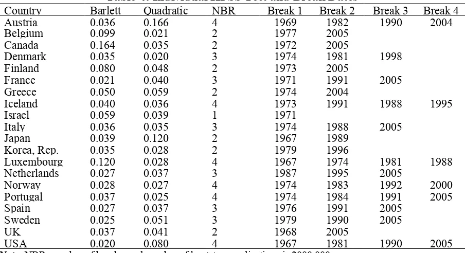
On the other hand, the allowance of structural breaks from the individual KPSS unit rot test shown in Table 4 suggest that the null hypothesis of stationarity is rejected at the 5% level of significance for all series except Belgium, Luxembourg, Canada and Finland.
Table 4: Individual KPSS Test and Break Dates
Country Barlett Quadratic NBR Break 1 Break 2 Break 3 Break 4 Austria 0.036 0.166 4 1969 1982 1990 2004 Belgium 0.099 0.021 2 1977 2005
Canada 0.164 0.035 2 1972 2005
Denmark 0.035 0.020 3 1974 1981 1998 Finland 0.080 0.048 2 1973 2005
France 0.021 0.040 3 1971 1991 2005 Greece 0.050 0.059 2 1974 2004
Iceland 0.040 0.036 4 1973 1991 1988 1995 Israel 0.059 0.039 1 1971
Italy 0.036 0.035 3 1974 1988 2005 Japan 0.039 0.120 2 1967 1989
Korea, Rep. 0.035 0.028 2 1979 1996
Luxembourg 0.120 0.028 4 1967 1974 1981 1988 Netherlands 0.027 0.037 3 1987 1995 2005
Norway 0.028 0.027 4 1974 1983 1992 2000 Portugal 0.037 0.025 4 1974 1984 1991 2005 Spain 0.027 0.037 3 1976 1991 2005
Sweden 0.025 0.051 3 1979 1990 2005 UK 0.037 0.041 2 1968 2005
USA 0.020 0.080 4 1967 1981 1990 2005
Note: NBR: number of breaks, and number of bootstrap replications is 2000.000
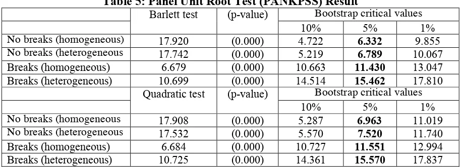
The PANKPSS panel stationarity test with structural breaks and without structural breaks is presented in Table 5 for the options of homogeneity and heterogeneity of long-run variance with their asymptotic critical values. The p-value of the test statistics given in parentheses is 0.000 for both the Bartlett and the Quadratic test regardless of heterogeneity or heterogeneity in the long-run variance estimate. The results show that the null hypothesis of panel stationarity is strongly rejected for homogenous and heterogeneous variance options. We should be careful about our cross-section independency assumption. Because this panel statistics does not take into account the cross-section dependency between individuals in the panel. However, this assumption is not so realistic in a globalized world where the shocks overpass the borders of the economies (Carrion-i Silvestre et al, 2005). Considering this dependency property, PANKPSS test statistics are compared with computed bootstrap critical values with 2000 replications, because we assume cross section independency for the panel. However, our conclusions remain unchanged when using these critical values. Statistics given in Table 5 are bigger than bootstrap critical values at the 5% significance level so that for the case of homogeneous and heterogeneous variance the null hypothesis of stationarity in the panel is rejected.
All these results indicate that per capita GDP series is non- stationary. This means that any shock given to per capita GDP is not short-lived, in contrast it is permanent. In other words, the impact of shocks to the per capita is not temporary and sooner or later per capita series will not return to its long-run equilibrium point.
Table 5: Panel Unit Root Test (PANKPSS) Result
Barlett test (p-value) Bootstrap critical values 10% 5% 1%
No breaks (homogeneous) 17.920 (0.000) 4.722 6.332 9.855
No breaks (heterogeneous 17.742 (0.000) 5.219 6.789 10.067 Breaks (homogeneous) 6.679 (0.000) 10.663 11.430 13.047 Breaks (heterogeneous) 10.699 (0.000) 14.514 15.462 17.810
Quadratic test (p-value) Bootstrap critical values 10% 5% 1%
No breaks (homogeneous 17.908 (0.000) 5.287 6.963 11.019
No breaks (heterogeneous 17.532 (0.000) 5.570 7.520 11.740 Breaks (homogeneous) 6.684 (0.000) 10.727 11.551 12.994 Breaks (heterogeneous) 10.725 (0.000) 14.361 15.570 17.837
The number of break points has been estimated using the LWZ information criteria allowing for a maximum of m = 5 structural breaks. The long-run variance is estimated using both the Bartlett and the Quadratic spectral kernel with automatic spectral window bandwidth selection as in Carrion et al. (2005), Andrews (1991), Andrews and Monahan (1992) and Sul et al. (2003). The number of bootstrap replications selected is 2000 as in Carrioni et al. (2005).
5. Conclusion. In this stud, we examine whether or not the per capita real GDP of 20 high- income OECD countries can be modelled as a stationary process for the period of 1961 to 2012. We have applied panel data stationarity test developed by Carrion-i-Silvestre et al. (2005) allowing multiple structural breaks in different dates under the null hypothesis of stationarity. Moreover, we apply individual time series unit root test with and without structural break, and the first generation panel unit root tests allowing cross section independency are also applied to the data set.
Empirical results indicate that per capita GDP series is non- stationary for many OECD countries. This means that any shock given to per capita GDP is not short-lived, in contrast it is permanent. In other words, the impact of shocks to the per capita is not temporary and later per capita series will not return to its long-run equilibrium point, i.e. it is not converging to its long-run level.
References
Ahmed, H.A. , Uddin, G.S. and Ozturk, I. (2012), Is Real Gdp Per Capıta Statıonary For Bangladesh? Empırıcal Evıdence From Structural Break, Actual Problems Of Economıcs; 2012, 128, p332-p339, 8p.
Andrews, D.W. K. (1991). Heteroskedasticity and autocorrelaction consistent covariance matrix estimation. Econometrica 59, 817–58.
Andrews, D.W. K. and J. C. Monahan (1992). An improved heteroskedasticity and autocorrelation consistent autocovariance matrix. Econometrica 60, 953–66.
Carrion-i-Silvestre, J., Del Barrio-Castro, T. and Lopez- Bazo, E. (2005) Breaking the panels: an application to the GDP per capita, Econometrics Journal, 8, 159–75.
Chang, H. L., Shen, P. L., and Su, C. W. (2013). Are real GDP levels nonstationary across Central and Eastern European countries?. Baltic Journal of Economics, (1), 99-108.
Chang, T., Chang, H., Chu, H. and Wei, C. (2006). Is per capita real GDP stationary in African countries? Evidence from panel SURADF test. Applied Economics Letters, 13, 1003– 1008
Christopoulos DK (2006) Does a non-linear mean reverting process characterize real GDP movements. Empir Econ 31:601–611.
Dickey, David A., and Wayne A. Fuller (1979). "Distribution of the estimators for autoregressive time series with a unit root." Journal of the American statistical association
74.366a: 427-431.
Fleissig, A. and Strauss, J. (1999) Is OECD real per capita GDP trend or difference stationary? Evidence from panel unit root tests. Journal of Macroeconomics, 21,673–90.
Guloglu, B., & Ivrendi, M. (2010). Output fluctuations: transitory or permanent? the case of Latin America. Applied Economics Letters, 17(4), 381-386.
Hadri, K. (2000). Testing for stationarity in heterogeneous panel data. Econometrics Journal 3, 148–61.
Im, K., Pesaran, H. and Shin, Y. (2003) Testing for unitroots in heterogenous panels,
Journal of Econometrics,115, 53–74.
Kitov, I., Kitov, O., & Dolinskaya, S. (2009). Modelling real GDP per capita in the USA: cointegration tests. Journal of Applied Economic Sciences, Spiru Haret University, Faculty of Financial Management and Accounting Craiova, 4(1), 7.
Kwiatkowski, D., P. C. B. Phillips, P. J. Schmidt andY. Shin (1992). Testing the null hypothesis of stationarity against the alternative of a unit root: How sure are we that economic time series have a unit root. Journal of Econometrics, 54, 159–78.
Levin, A., Lin, C., Chu, J. and Shang, C. (2002) Unit roots tests in panel data:asymptotic and finite sampleproperties, Journal of Econometrics, 108, 1–24.
Narayan, P. K., & Narayan, S. (2010). Is there a unit root in the inflation rate? New evidence from panel data models with multiple structural breaks. Applied economics, 42(13), 1661-1670.
Narayan, P. K. (2008). Is Asian per capita GDP panel stationary?. Empirical economics, 34(3), 439-449.
Maddala, G. S. and Wu, S. (1997) A comparative study ofunit root tests with panel data and a new simple test,Ohio State University, Working Paper.
Özturk, I. and Kalyoncu, H.(2007). Is Per Capita Real GDP Stationary in the OECD Countries?, Ekonomiski Pregled, 58 11, 2007, 680-688
Rapach, D. E. (2002). Are real GDP levels nonstationary? Evidence from panel data tests. Southern Economic Journal, 473-495.
Smyth, R., & Inder, B. (2004). Is Chinese provincial real GDP per capita
Sul, D., P. C. B. Phillips and C. Y. Choi (2003). Prewhitening bias in HAC estimation. Cowles foundation discussion paper num. 1436.
Su, Chi-Wei, et al. "IS Per Capita Real GDP Stationary in China¡ Evidence Based on A Panel SURADF Approach." Economics Bulletin 3.31 (2007): 1-12
Zivot, Eric, and Donald W. K. Andrews. (2002) "Further evidence on the great crash, the oil-price shock, and the unit-root hypothesis." Journal of Business & Economic Statistics