Munich Personal RePEc Archive
Efficacy of a bidder training program:
lessons from LINC
De Silva, Dakshina G. and Hubbard, Timothy P. and
Kosmopoulou, Georgia
Lancaster University, Colby College, National Science Foundation
University of Oklahoma
30 July 2015
Online at
https://mpra.ub.uni-muenchen.de/65862/
Efficacy of a Bidder Training Program: Lessons from LINC
∗
Dakshina G. De Silva
†Timothy P. Hubbard
‡Georgia Kosmopoulou
§July 30, 2015
Abstract
In an effort to accommodate a change in the U.S. Federal Highway Administration’s goals towards “race-neutral methods” concerning the involvement of Disadvantaged Business Enterprises in pro-curement contracting, the Texas Department of Transportation created a Learning, Information, Networking and Collaboration (LINC) bidder training program. We examine the costs, benefits, and efficacy of this program using ten years of data, employing firm-specific bidding patterns with participation dates. We distinguish between ineligible firms as well as eligible firms that undergo training and those that don’t, to consider a number of different empirical models which allow for potential asymmetries across these bidder groups.
JEL Classification: D44, H57, R42.
Keywords: auctions, bidder training, disadvantaged business enterprises.
∗We are grateful to Jorge Balat, Tim Dunne, Philippe Gagnepain, Matt Gentry, Brent Hickman, Han Hong, Fabio
Miessi, Jimmy Roberts, and Steve Tadelis for valuable discussions at different stages of this project. We would also like to acknowledge participants at the International Conference on Contracts, Procurement and Public-Private Agreements, the International Industrial Organization Conference, the Workshop on Procurement and Contracts at the University of Mannheim, the Brazilian Conference Series on Public Procurement and Concession Design, the Lancaster University Conference on Auctions, Competition, Regulation, and Public Policy and seminar participants at Copenhagen Business School, Maastricht University, Oberlin College, the University of Guelph, the University of Maine, and the University of New Hampshire for helpful comments. Lastly, we thank the Texas Department of Transportation for providing the data. Any opinions, findings, and conclusions or recommendations expressed in this material are those of the authors and do not necessarily reflect the views of the National Science Foundation.
†Department of Economics, Lancaster University Management School, Lancaster LA1 4YX, UK; email:
‡Department of Economics, Colby College, 5242 Mayflower Hill Drive, Waterville, ME 04901, USA; email:
§National Science Foundation, 4201 Wilson Blvd, Arlington, VA 22230 and Department of Economics, University of
1
Introduction
The U.S. Federal Highway Administration (FHWA) has used government policies since at least the
early 1980’s to encourage minority participation in procurement contracting. Many states employ
bid preference programs, which discount the bids of qualified firms for the purpose of evaluation.
Other programs require government agencies to set aside a certain percentage of a contract to be
subcontracted out to disadvantaged business enterprises (DBEs) or other qualified firms. Over the
decades and largely in response to court decisions (see, for example, the Supreme Court’s 1999 ruling
in Adarand v. Pe˜na, U.S. Report 515 U.S. 200), the nature and administration of DBE programs has
changed. While they still retain their basic structure, the goal of firm participation is now described as
being “aspirational.” Individual state agencies that administer the programs, are asked to achieve as
much of the goal as possible by “race-neutral methods” before employing other race-conscious policies.
For example, qualified DBE firms are not simply determined by belonging to a particular demographic
group (e.g., being owned by a minority, veteran, or woman) but also by their economic circumstances
(e.g., small businesses). The overall regulatory response of the FHWA was to tailor programs to meet
the Court’s objections.
In response to the shift in the disposition of FHWA policy, the Texas Department of Transportation
(TxDOT) created its own Learning, Information, Networking, Collaboration (LINC) training program
in 2001 to mentor eligible firms interested in doing business with TxDOT.1 Texas has the second
largest state economy in the U.S. and a diverse population with 37.62% of its residents identifying as
Hispanic and 11.94% as Black in the 2010 Census. The intent of the LINC program is to maintain and
support the role qualified firms play in the TxDOT procurement process by providing information,
networking opportunities, project management, and training sessions. The program allows firm owners
to improve their knowledge and project management skills, thus, increasing the chances for success
without explicitly constraining the decision-making process. During our ten-year sample period which
spans September 1997 to August 2007, the total value of contracts awarded to LINC-eligible bidders 1
was $2.04 billion. We examine the impact of the LINC program on participation, bidder behavior,
chances for success, and the cost structure of qualified bidders acting as primary contractors. The
LINC program description states that the targeted firms are “critical to economic competitiveness in
the Transportation industry.” As such, we also consider whether the LINC program might improve
retention of such firms in the long-run for this industry.
We find the most convincing effects LINC has on bidders is with respect to bidding behavior—
LINC-trained bidders behave more aggressively than firms that are not eligible for the program as well
as those that are eligible but have not undergone the training program. In addition, the interest of a
LINC-trained firm in a project generates an indirect competition effect in which ineligible firms (our
most frequently-observed class of bidders) behave more aggressively than they otherwise would have.
The lower bids carry through to generate cost-savings for TxDOT in two ways: first, when
LINC-trained firms win their bids are lower, on average, than those of all other firms. Second, when other
firms compete at auctions which attract interest from LINC-trained firms, the average winning bid is
also lower. These two channels generate substantial savings for the state—even our most conservative
estimates involve millions of dollars saved. We find LINC-trained firms that then win auctions maintain
similar Lerner indexes to other firms. Moreover, eligible firms that do not get trained are more likely
to exit the industry than firms that are not eligible, but this effect goes away for firms that graduate
from the LINC program.
The efficacy of other class-specific preference policies on procurement costs have been examined by
a number of researchers with varying conclusions. Several papers deal with bid preference schemes.2
Denes [1997] compared bids submitted between solicitations restricted to small businesses and
unre-stricted solicitations, finding that bids are no higher in reunre-stricted settings. Marion [2007] found that
in data from California auctions for road construction contracts, the price paid by the state was 3.8
percent higher for auctions which used preferences. Krasnokutskaya and Seim [2011] also analyzed
bid preference programs in California highway procurement contracts and found that the preferential 2
treatment of small businesses creates losses in efficiency but no change in the overall cost of
procure-ment.
While bid preference policies introduce an asymmetry among bidders (even if bidders draw costs
from the same distribution), the potential for efficiency distortions stems from a different source for
programs setting minority subcontracting goals. These programs are often used in federal
procure-ment contracts and may constrain the make-or-buy decision of prime contractors. Distortions may
occur because of potentially less efficient production of tasks by subcontractors compared to the prime
contractor (relative to an unrestricted setting) or due to changes in competition intensity in the
sub-contracting market. Marion [2011] used data from the California Department of Transportation to
show that the subcontracting goals set for highway construction contracts in California raise DBE
usage significantly, so that the constraints appear to bind. In fact, Marion [2009] found that after
Cal-ifornia’s Proposition 209 was passed (which prohibited DBE subcontracting goals concerning race or
gender), state-funded contracts realized a 5.6 percent fall in prices relative to federally-funded projects
which still involved subcontracting goals. De Silva et al. [2012] evaluated the impact of a federal
subcontracting policy years after its original implementation and found that minority subcontracting
goals have not increased the procurement cost in Texas.
To our knowledge, we are the first to study the effects of a bidder-training program. We have
contacted representatives at every U.S. state’s Department of Transportation office and have learned
two things: first, these programs are quite common as more than thirty states have in place a program
with many of these elements; second, Texas seems to be one of the first states to introduce such a
program and its program seems to be one of the largest in terms of participation. In our
correspon-dence with employees at state offices we have learned that these programs often go by different names
(e.g., Calmentor in California, Connect2DOT in Colorado, and Mission 360oin Rhode Island) and are
often defined as mentor-prot´eg´e programs which are administered through economic or local
develop-ment offices. Most programs have bidder training, formal develop-mentoring, educational seminars, outreach
components such as trade shows and business fairs, technical assistance, financial and management
effective business development by improving the performance of trained firms, ultimately hoping for a
higher survival rate of such firms.
In general, such training programs seem to be on the rise. Some states have either implemented new
programs (e.g., the Oklahoma Department of Transportation’s Small Enterprise Training Program) or
are re-emphasizing or revamping old programs (e.g., the Washington Department of Transportation
recently expanded its program from targeting minority- and women-owned firms to include small
businesses in general), and a number of representatives for states that do not currently have any
programs indicated that they felt such opportunities would be a good idea. Moreover, these programs
are not unique to Department of Transportation—the leading inspiration for such programs seems
to be the Stempel Program for the Port of Portland in Oregon.3 Given the prevalence and interest
in such training programs, we hope our work has important policy implications as there is potential
for our findings to suggest alternative policies to meet the FHWA’s original goals in a way that can
actually generate clear cost savings (benefits). The only costs for the state are administrative salaries
and expenses associated with organizing LINC-related sessions. We have obtained expense data that
reports LINC costs for fiscal years 2005 to 2012 which show that the program costs the state about
$200,000 per fiscal year.4 In what follows, we hope to shed light on the potential benefits to be had from
such a program either through participation, bidding, efficiency improvements, and/or firm retention.
In the next section, we describe our TxDOT data and first examine what drives a qualified firm
to participate in the program. In Section 3, we investigate whether trained firms are more likely to
bid on a contract once they hold the plans, as well as whether they are more likely to win a contract
given they’ve chosen to bid. Linking the former probability concerning a firm’s choice with the latter
probability which involves an outcome is firm behavior. As such, we present a number of empirical
models to document and help us interpret observed bidding patterns. Importantly, we can identify how
bidding changed after program completion and evaluate effects the LINC program has had on winning 3
See the very informative Wisconsin Department of Transportation [2010] report which summarized and surveyed how such programs have been operated in the U.S. and the Associated General Contractors of America’s website: http://www.agc.org/cs/industry topics/additional industry topics/the stempel plan for additional details on such pro-grams.
4
bids. Given what we can observe in the data, we also explore other ways in which LINC training
might have changed firm behavior which have some backing in the auctions literature. Because these
dimensions do not suggest changes that result from LINC, we consider whether something we cannot
directly observe in the data might have changed in an important way. Specifically, in Section 4, we
present a structural model which allows us to speak about potential changes to firms’ (unobserved)
cost structures, the efficiency of the auctions, and market power in the industry. The results and
insights from such estimates live in Section 5. LINC-eligible firms have lower average costs and their
cost distributions (trained or untrained) are significantly different from ineligible firms. However, when
comparing distributions within the group of LINC-eligible firms, we do not find a statistical difference
in the latent distribution of costs based on whether the firm is trained or not. In Section 6, we consider
whether firm survival in the industry has been affected by participation and, lastly, in Section 7, we
summarize our work and conclude.
2
The LINC Program
Our primary focus is on how the bidding behavior might change as a result of the LINC program.
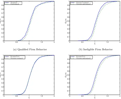
A snapshot of bidding patterns observed in the data helps motivate this investigation. In Figure 1,
we present four subplots containing empirical distribution functions of relative bids—the observed
bids submitted by the firms normalized by the state’s engineering cost estimate for the project. We
condition on the engineer’s estimate so that the bids are at least comparable across auctions. Auction
theory says that bidding behavior changes with the number of participants at auction. As such, we
restrict data for this set of figures to auctions for which we observe five bidders tendering offers. Keep
in mind that, at procurement auctions, low bids are (aggressive behavior is) good for the state which
is seeking to have a task completed at the lowest possible cost. The subplots leverage distinctions in
the class of the competing firms based on whether they are eligible for and whether they participated
in the LINC program by the time their bids were tendered.
In subplot 1a, we consider the behavior of firms that are eligible for the LINC program at five-bidder
0 0.5 1 1.5 2 0 0.1 0.2 0.3 0.4 0.5 0.6 0.7 0.8 0.9 1 b ˆ G B ( b )
Tr aine d Unt r aine d
(a) Qualified Firm Behavior
0 0.5 1 1.5 2
0 0.1 0.2 0.3 0.4 0.5 0.6 0.7 0.8 0.9 1 b ˆ G B ( b )
Ve r s us t r aine d Ve r s us unt r aine d
(b) Ineligible Firm Behavior
0 0.5 1 1.5 2
0 0.1 0.2 0.3 0.4 0.5 0.6 0.7 0.8 0.9 1 b ˆ G B ( b )
Sy mme t r ic Ve r s us t r aine d
(c) Ineligible Firm Behavior: Symmetric vs. Asymmet-ric with Trained
0 0.5 1 1.5 2
0 0.1 0.2 0.3 0.4 0.5 0.6 0.7 0.8 0.9 1 b ˆ G B ( b )
Sy mme t r ic Ve r s us unt r aine d
[image:8.612.97.502.197.528.2](d) Ineligible Firm Behavior: Symmetric vs. Asym-metric with Untrained
In contrast, in subplot 1b, we consider the behavior of firms that are not eligible for the LINC program
and consider how they behave at auctions involving other ineligible firms along with at least one
LINC-eligible firm. The figure suggests that these firms behave more aggressively when a LINC-trained firm
is present at auction than when an eligible, but untrained firm is present. In subplots 1c and 1d,
we consider again only the behavior of ineligible firms, but compare their bids at symmetric auctions
(comprised only of ineligible firms) with their behavior at asymmetric auctions (comprised of ineligible
firms and at least one LINC-eligible firm). Subplot 1c, shows that if the auction is asymmetric because
a LINC-trained firm is present, behavior is not distinguishable from behavior at symmetric auctions.
However, subplot 1d, shows that if the auction is asymmetric because a LINC-eligible, but untrained
firm is present, bids of ineligible firms are less aggressive than their behavior at symmetric auctions.
Together, these figures suggest a pattern: once firms have undergone LINC training, they appear to
behave more aggressively (1a); ineligible firms (constituting the majority of the state’s bidding firms),
behave more aggressively when facing LINC-trained rivals (1b) than when facing untrained firms;
ineligible firms’ bids appear no different when they face only peer ineligible firms compared to when a
LINC-trained rival participates (1c), but if the rival is untrained, behavior is less aggressive (1d). We
investigate this story rigorously in our empirical work by modeling firms’ decisions and accounting for
many other factors that are not accounted for in these motivating figures.5
We continue our investigation of the effects of the LINC program by describing our data and
determining what might drive qualified firms to participate in LINC. Note that, we take as given,
the set of eligible firms—these, by requirement of the LINC program, must be firms that have been
certified as a DBE, HUB, or SBE for at least one year.6
5
Kolmogorov–Smirnov tests suggest that the empirical distributions are significantly different at the one-percent level in subplots 1b and 1d; the distributions in subplot 1a are significantly different at the ten-percent level (while visually a difference appears, the underlying sample sizes are smaller than in the other subplots); we fail to reject a null that the distributions are the same in subplot 1c, perhaps not surprisingly as the two nearly overlap each other.
6
2.1
Data Description
In our analysis, we use data from regularly-scheduled TxDOT highway procurement auctions conducted
between September 1997 and August 2007. Data from September 1997 to August 1998 are used to
create bidder-specific histories such as a measure of workload commitment (commonly referred to in
the auctions literature as backlog). Thus, our empirical analysis in what follows employs the data from
September 1998 through August 2007. Prior to bidding, all bidders learn the location and the detailed
project description, the estimated number of days to complete the project, the engineer’s estimate of
the cost of executing the project, and the list of contractors who purchased the documents providing
the initial plan description (the plan holders). Projects are awarded using the low-price, sealed-bid
(procurement) auction format. The bidding process opens a minimum of 28 days after the plan for a
project is posted. When the bidding period expires, the offers submitted by each bidder are revealed
and the winner is announced. The winning bidder is determined solely by price—the lowest bidder is
awarded the right to complete the respective task for the government. For each contract, we observe
the identities of the firms that requested plans, the identities of all firms that tendered a bid along
with the amount of each bid, as well as the engineer’s cost estimate, projected time to complete the
contract, and details concerning the tasks each contract requires. We complement these data with
firm-specific LINC-eligibility and LINC-participation data and we construct, using each firm’s past
bidding behavior, other variables that might be important in driving observed behavior.
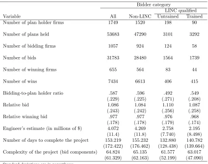
In Table 1, we present sample summary statistics for the full sample, for ineligible/non-qualified
(non-LINC) firms, and for LINC-eligible firms. We partition the LINC-eligible firms into two groups:
untrained and trained. The untrained firms include firms that are eligible but choose not to participate
in the program and those who eventually get trained, but are observed in our data before training.
In the full sample, we find 1749 unique firms holding plans. Of those firms, 229 are LINC-qualified
prime bidders, 90 of which have participated in the LINC program.7 In our sample period, 58 LINC
7
Table 1: Summary statistics
Bidder category
LINC qualified
Variable All Non-LINC Untrained Trained
Number of plan holder firms 1749 1520 198 90
Number of plans held 53683 47290 3101 3292
Number of bidding firms 1057 924 124 58
Number of bids 31783 28480 1564 1739
Number of winning firms 655 564 83 44
Number of wins 7434 6613 406 415
Bidding-to-plan holder ratio .587 .596 .492 .549 (.229) (.225) (.271) (.208)
Relative bid 1.086 1.084 1.110 1.087
(.243) (.242) (.256) (.258)
Relative winning bid .977 .977 .976 .968
(.178) (.178) (.179) (.174) Engineer’s estimate (in millions of $) 4.072 4.269 2.758 2.195 (11.4) (11.8) (7.740) (8.498) Number of days to complete the project 153.219 155.232 132.880 140.782 (172.422) (176.462) (128.438) (139.664) Complexity of the project (bid components) 64.824 65.135 61.577 63.017
(61.329) (62.163) (52.199) (47.090) Standard deviations are in parentheses.
participants went on to eventually submit bids (constituting 1739 bids) and we observe 44 of them
winning at least one contract. The bidding-to-plan holder ratio is a measure of bidding frequency of
those indicating interest in a project by purchasing a plan. When considering this ratio, participation
rates for ineligible firms are about ten percent higher than those for LINC-qualified, but untrained
firms. LINC training cuts this disparity in half. Note too, that if the number of wins is normalized by
the number of bids, the winning-to-bidding ratio is fairly consistent across the categories. A potentially
important difference is that the number of LINC-trained firms submitting these winning bids is just
over half that of the number of untrained winners, indicating that training might improve success rates
The table suggests some potential for government savings. Before training, LINC-qualified firms
submit relative bids that are about two percent higher than traditional firms, though this difference
goes away after LINC training. We also see that after training, LINC bidders’ relative winning bids are
about one percent lower than those of other groups. The last three rows of the table indicate the type
of contracts in which bidding occurs may play an important role. These variables proxy for the average
size or complexity of the projects on which bids are submitted. LINC-qualified bidders, on average, bid
on projects that are estimated by state engineers to cost about $1.5 million less than projects non-LINC
firms bid on (and this difference increases after training). We also see that projects undertaken by
qualified bidders take 15–20 days less, on average, than those by ineligible bidders. Qualified bidders
also undertake projects that are typically less complex in that they have fewer components. Taken
together, the table suggests potentially important changes to bidder behavior, perhaps from LINC
participation. We will account for these in our empirical work that follows to understand the effects
of this program.
2.2
LINC Participation
Before considering the effects of LINC training, we first consider what might drive eligible firms to
participate in the program. Specifically, we consider a probit model using monthly data to explain the
probability of participating. The first time a LINC-eligible firm requests plans, the firm is assigned a
response variable taking a value of zero (having not participated in LINC). If the firm completes the
LINC program, the response variable changes to a one and then the firm is dropped from the panel.
We restrict attention to LINC-qualified entrants since 2001, the inception year of the LINC program
as firms that entered earlier did not have the opportunity to participate, even if they would have been
willing to. We also only consider months in which qualified firms had the opportunity to participate
in LINC.
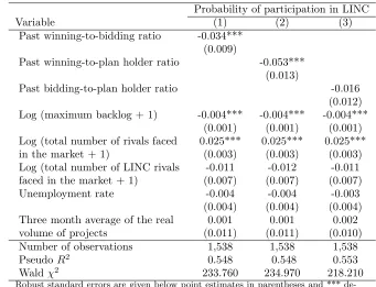
In Table 2, we present the estimates of three probit regressions as marginal effects. The models
differ by various measures of a given firm’s experience which is captured by the past winning-to-bidding,
LINC-eligible firm, the less likely the firm is to participate in LINC. For example, model (1) suggests that a
one-unit increase in a firm’s winning-to-bidding ratio means the firm is 3.4% less likely to participate in
the LINC training program. The lower experience effects are more salient for firms that have won often
in the past compared to those that have garnered experience primarily through simply participating
(bidding) in auctions as the past bidding-to-plan holder ratio is negative but not significant in model
[image:13.612.133.474.249.510.2](3).8
Table 2: LINC Training Participation Decision
Probability of participation in LINC
Variable (1) (2) (3)
Past winning-to-bidding ratio -0.034*** (0.009)
Past winning-to-plan holder ratio -0.053*** (0.013)
Past bidding-to-plan holder ratio -0.016 (0.012) Log (maximum backlog + 1) -0.004*** -0.004*** -0.004***
(0.001) (0.001) (0.001) Log (total number of rivals faced 0.025*** 0.025*** 0.025*** in the market + 1) (0.003) (0.003) (0.003) Log (total number of LINC rivals -0.011 -0.012 -0.011 faced in the market + 1) (0.007) (0.007) (0.007) Unemployment rate -0.004 -0.004 -0.003
(0.004) (0.004) (0.004) Three month average of the real 0.001 0.001 0.002 volume of projects (0.011) (0.011) (0.010) Number of observations 1,538 1,538 1,538
PseudoR2 0.548 0.548 0.553
Waldχ2 233.760 234.970 218.210
Robust standard errors are given below point estimates in parentheses and *** de-notes statistical significance at the 1% level.
In all models, we include a set of controls to capture economic conditions facing a firm,
character-izing the market, or expected to obtain in the future. The maximum backlog and number of rivals
faced are firm-specific—the maximum backlog capturing the size (capacity) of the firm and the
num-ber of rivals being the numnum-ber of unique plan holders a firm has faced in its previous participation
in auctions. If the firm has existing projects it is slightly less likely to participate. This finding is 8
statistically significant and robust across specifications. The magnitude of this effect is much lower
than the effects from increased competition. Firms that faced a larger number of rivals in the past are
more likely to participate in the program. The monthly unemployment rate in Texas is included as a
control, though it is not significant nor is the average value of potential projects which is computed
as a three-month moving average value of projects offered by TxDOT. Having considered what might
determine a firm’s participation decision, we now consider the effects of LINC training.
3
The Effects of LINC Training
While the summary statistics in Table 1 suggest some interesting patterns, they provide little direct
evidence of how entry, bidding, and winning may have been affected by the LINC program as we saw
the types of contracts firms chose to bid on were different across the categories of firms. The firm
characteristics driving LINC participation suggest important controls that must be accounted for in
going forward—namely a bidder’s experience, backlog, and the competitiveness of an auction. In this
section, we attempt to control for factors that may be varying across the sample periods, auctions, and
bidders in order to better gauge the effects the LINC program has had on this market. We partition
our analysis into two types of results: the first concerns probabilities of actually bidding and winning
while the second concerns the levels of bids and winning bids.
3.1
Likelihood of Bidding and Winning
First, we examine whether participation in the LINC program affected the entry patterns for
LINC-qualified bidders. To consider this, we estimated probit models characterizing the probability of bidding
in a given auction, conditional on the firm holding plans, and present estimation results in columns
(1) and (2) of Table 3.9 Our main interest is in the coefficient of the dummy variable “LINC-trained
firm” which takes a value of one if the firm is a LINC-qualified firm and has completed the training
program and takes a value of zero otherwise. Note that “LINC-qualified, but untrained firm” is also 9
a dummy variable that takes a value of one if the bidder is in fact a LINC-qualified firm, but instead
indicates that the firm has not participated in the training program, and is zero otherwise. Again,
this may involve firms that were invited but chose not to participate in the program and firms that
eventually participated in LINC, but we observe them in our data before they participated. While
these variables capture average differences in the participation and success between LINC-eligible and
ineligible firms, as well as allow us to understand the direct effect of the LINC training program, we
are also interested in any indirect effects that might result. As such, we include a dummy variable
“Interest from LINC-trained firm” to capture how the behavior of rival firms might change when a
LINC-trained firm shows interest in a project. This takes a value of one when a LINC-trained firm
holds plans for a given auction and measures the indirect effect of the LINC program.10 We consider
our full (September 1998 to August 2007) sample in models (1) and (2) and restrict attention to only
the LINC-qualified sample in model (3).
Most of our other independent variables serve as a set of controls and involve accounting for things
that are commonly used in the auctions literature. They can be categorized as representing auction,
firm-specific, rival, and market characteristics. As project characteristics, we include the estimated
cost of the project provided by state engineers, the number of potential rivals (plan holders), the days
to complete a project, the complexity of a project as measured by the number of bid components,
the project’s materials shares, and the project division identified by TxDOT. The firm-specific
char-acteristics involve the share of the firm’s capacity utilized, the logarithm of the firm’s distance to the
project location, a dummy variable that takes the value of one if the firm has an ongoing project in the
same county as the current project county, and the number of past bids. Proximity and concurrent
involvement in local projects can reduce moving costs and create the opportunity to share resources
more effectively across projects. The number of past bids is used to capture any experience gathered
from prior bidding. As rival characteristics, we include the average rivals’ past winning-to-plan holder 10
ratio, rivals’ minimum backlog, and the logarithm of the closest rival’s distance to the project location.
Finally we include a set of time dummies to control for market fluctuations. A detailed description of
[image:16.612.92.526.183.573.2]these variables is provided in the Appendix.
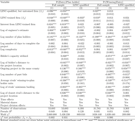
Table 3: Results for Probability of Entry and Winning Conditional upon Entry
Variable Pr[Entry|Plan holder] Pr[Winning|Entry]
Full sample LINC-qualified Full sample LINC-qualified
(1) (2) (3) (4) (5) (6)
LINC-qualified, but untrained firm (β1) -0.096*** -0.050*** 0.027** 0.013
(0.010) (0.010) (0.012) (0.012)
LINC-trained firm (β2) -0.048*** -0.049*** -0.033* 0.019* 0.013 0.024
(0.009) (0.009) (0.019) (0.011) (0.011) (0.023) Interest from LINC-trained firm 0.024*** 0.019*** 0.022 -0.007 -0.005 -0.027 (0.005) (0.005) (0.017) (0.006) (0.006) (0.019) Log of engineer’s estimate 0.008** 0.009*** 0.006 -0.002 0.004 -0.030***
(0.003) (0.003) (0.010) (0.004) (0.004) (0.012) Log number of plan holders -0.185*** -0.151*** -0.133*** -0.199*** -0.204*** -0.162***
(0.007) (0.008) (0.025) (0.008) (0.008) (0.028) Log number of days to complete the 0.002 0.004 -0.022 -0.001 -0.001 0.013
project (0.004) (0.004) (0.014) (0.005) (0.005) (0.016)
Log complexity -0.013*** -0.040*** -0.052*** 0.004 0.001 0.038*** (0.004) (0.004) (0.013) (0.005) (0.005) (0.014) Bidder’s capacity utilized 0.020** -0.024 -0.074*** -0.129***
(0.010) (0.033) (0.011) (0.037) Log of bidder’s distance to -0.045*** -0.049*** -0.021*** -0.016**
the project location (0.002) (0.007) (0.002) (0.007)
Ongoing project in the same county 0.136*** 0.166*** 0.078*** 0.058*** (0.006) (0.019) (0.006) (0.022) Log number of past bids 0.040*** 0.071*** -0.007*** -0.015* (0.001) (0.006) (0.002) (0.008) Average rivals’ winning-to-plan -0.336*** -0.525*** -0.539*** -0.514***
holder ratio (0.050) (0.161) (0.052) (0.174)
Log of rivals’ minimum backlog -0.003*** -0.005*** -0.001*** -0.003* (0.000) (0.001) (0.000) (0.001) Log of closest rival’s distance to the 0.026*** 0.030*** 0.020*** 0.001
project location (0.002) (0.008) (0.003) (0.009)
Time effects Yes Yes Yes Yes Yes Yes
Material shares Yes Yes Yes Yes Yes Yes
Project division effects Yes Yes Yes Yes Yes Yes
Number of observations 53,683 53,683 6,393 31,783 31,783 3,303
PseudoR2 0.049 0.094 0.120 0.035 0.051 0.082
Waldχ2 2,660.680 5,426.230 889.010 1638.440 1,639.440 289.090
χ2test probability:β
1=β2 0.002 0.931 0.608 0.986
Robust standard errors are given below point estimates in parentheses and *, **, and *** denote statistical significance at the 10%, 5%, and 1% level, respectively.
The results indicate that LINC-eligible firms, relative to the ineligible firms (our omitted group)
are 4.8–9.6% less likely to bid in a given auction. The results in model (1) include only
entry. However, when firm-specific and rival-specific characteristics are controlled for, the difference
disappears: using the estimates in columns (1) and (2), we test whether H0 : β1 = β2 against a
two-sided alternative and our results change dramatically as we fail to reject the null once the other
controls are added; however, when we restrict attention to the LINC-qualified sample in column (3),
the training dummy variable is significantly different from zero at the 10% level. The estimates indicate
that as the number of plan holders, project complexity, and a bidder’s distance to project location
increases, or when they are facing strong rivals, a firm’s probability of entering an auction decreases.
Bidders who have ongoing projects in the same bidding location (same county), those facing rivals
who are located farther away from a project site, or those who have bidding experience have a higher
probability of entry.
In models (4)–(6) of Table 3, we consider whether the probability of winning conditional on bidding
at an auction changes after a firm has graduated from the LINC program. Our results indicate that
once bidder- and rival-specific effects are controlled for, neither being qualified nor being
LINC-trained affects the chances of winning at auction. Bidders with higher capacity utilized, those located
farther from the project location, and those facing competitive rivals are less likely to win, while those
firms having ongoing projects in the same county appear more likely to win. Interestingly, experience
seems to work against the chances of winning for firms but this could be because experience tempers
firms from bidding too aggressively. Of course, the bidding behavior of firms and the question of
whether bidding has changed is driving the relationship between these two sets of empirical results—
something we explore further in the next subsection.
3.2
Bidding and Winning Bids
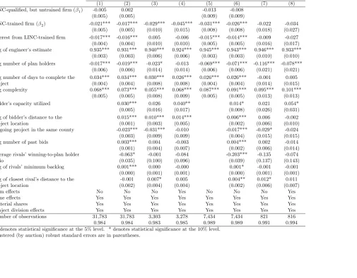
We examine next whether bidding has been affected by the LINC training program. In Table 4
we provide a set of least squares regression results for the full sample and the restricted sample of
LINC-qualified bidders. Specifically, in the first four columns we consider explaining variation in the
logarithm of all tendered bids while in the last four columns we restrict attention to the log of only
Table 4: Bid Regression Results
Variable Log of bids Log of winning bids
Full sample LINC qualified Full sample LINC qualified
(1) (2) (3) (4) (5) (6) (7) (8)
LINC-qualified, but untrained firm (β1) -0.005 0.002 -0.013 -0.008
(0.005) (0.005) (0.009) (0.009)
LINC-trained firm (β2) -0.021*** -0.017*** -0.029*** -0.045*** -0.031*** -0.026*** -0.022 -0.034
(0.005) (0.005) (0.010) (0.015) (0.008) (0.008) (0.018) (0.027)
Interest from LINC-trained firm -0.017*** -0.016*** 0.005 -0.006 -0.015*** -0.014*** -0.009 -0.027
(0.004) (0.004) (0.010) (0.010) (0.005) (0.005) (0.016) (0.017)
Log of engineer’s estimate 0.935*** 0.931*** 0.940*** 0.924*** 0.945*** 0.943*** 0.946*** 0.933***
(0.003) (0.003) (0.006) (0.006) (0.003) (0.003) (0.010) (0.010)
Log number of plan holders -0.017*** -0.019*** -0.023* -0.013 -0.069*** -0.071*** -0.116*** -0.078***
(0.006) (0.006) (0.014) (0.014) (0.006) (0.006) (0.021) (0.021)
Log number of days to complete the 0.034*** 0.034*** 0.030*** 0.026*** 0.026*** 0.026*** -0.001 0.005
project (0.004) (0.004) (0.008) (0.008) (0.004) (0.004) (0.014) (0.015)
Log complexity 0.068*** 0.073*** 0.055*** 0.068*** 0.087*** 0.091*** 0.095*** 0.101***
(0.005) (0.005) (0.008) (0.009) (0.005) (0.005) (0.013) (0.013)
Bidder’s capacity utilized 0.030*** 0.026 0.040** 0.014* 0.021 0.054*
(0.005) (0.016) (0.017) (0.008) (0.026) (0.031)
Log of bidder’s distance to the 0.015*** 0.010*** 0.014*** 0.006*** 0.006 -0.002
project location (0.001) (0.003) (0.005) (0.002) (0.006) (0.010)
Ongoing project in the same county -0.023*** -0.031*** -0.010 -0.017*** -0.029* -0.024
(0.003) (0.009) (0.009) (0.004) (0.015) (0.015)
Log number of past bids 0.003*** 0.004 -0.003 0.004*** 0.002 -0.014
(0.001) (0.004) (0.007) (0.002) (0.006) (0.014)
Average rivals’ winning-to-plan holder -0.063* -0.001 -0.084 -0.203*** -0.135 -0.074
ratio (0.035) (0.100) (0.096) (0.039) (0.137) (0.143)
Log of rivals’ minimum backlog 0.001*** 0.000 -0.000 0.001* -0.001 -0.001
(0.000) (0.001) (0.001) (0.000) (0.001) (0.001)
Log of closest rival’s distance to the -0.001 0.007* 0.005 0.004** 0.012* 0.011
project location (0.002) (0.004) (0.004) (0.002) (0.006) (0.007)
Firm effects No No No Yes No No No Yes
Time effects Yes Yes Yes Yes Yes Yes Yes Yes
Material shares Yes Yes Yes Yes Yes Yes Yes Yes
Project division effects Yes Yes Yes Yes Yes Yes Yes Yes
Number of observations 31,783 31,783 3,303 3,278 7,434 7,434 821 816
R2 0.984 0.984 0.983 0.985 0.989 0.989 0.991 0.994
** denotes statistical significance at the 5% level. * denotes statistical significance at the 10% level.
When all firms are considered, as in models (1) and (2), the omitted group is the
ineligible/non-LINC firms.11 There is no statistically significant difference in the bidding behavior of LINC-qualified,
but untrained firms and the ineligible firms. However, the estimate of the coefficient β2 indicates
that after completing LINC training, firms bid more aggressively compared to their pre-LINC-training
levels and relative to the ineligible firms. Specifically, LINC-trained firms bid 1.7% lower than other
vying firms. Perhaps as important is the indirect competition effect which here captures the bidding
behavior of firms that submit offers on projects which LINC-trained firms expressed interest in. When
that is the case, the bid is 1.6% lower on average. We have some confidence in this indirect competition
effect as we considered other models in which we included placebo-like effects.12 For example, if we
include a variable capturing whether plans for the auction were held by a LINC-qualified, but untrained
firm (either along with or instead of the one representing our indirect competition effect) it is never
statistically different from zero and is always smaller in magnitude, being at most 0.004 away from
zero. In short, on average, the training program seems to be generating aggressive bidding both directly
from the program’s graduates, and indirectly through more competitive behavior from rival firms when
LINC graduates hold plans for an auction.
The other coefficient estimates suggest patterns that are intuitively appealing. If there are more
plan holders at auction, if a firm has another project going on in the same county and can, perhaps,
generate synergistic benefits, or if the rivals have been more successful in past auctions, then lower
bids are tendered. If the size, length, or complexity of the project is larger/higher, then higher bids
are submitted. Likewise, higher bids obtain when bidders have used much of their capacity or if firms
are farther from the project location. All of these effects are statistically significant at the 1% level
even after controlling for time, project composition, and project division effects. While statistically
significant, a bidder’s experience and the rivals’ minimum backlog are both very small in magnitude.
Their signs indicate that having tendered many bids in the past or facing rivals with many ongoing
projects led a firm to tender higher bids on average. 11
We do not discuss extensively model (1) here, but present it to help give a baseline and to frame a bid homogenization procedure that we will later use.
12
In columns (3) and (4) of Table 4 we restrict attention to the subsample of bids generated by
LINC-qualified firms. As such, the omitted group now becomes the set of firms that opt not to
undergo training. Relative to this group of untrained, but eligible firms, LINC bidding is even more
competitive—the results suggesting bids that are 2.9% or 4.5% lower, depending on whether firm fixed
effects are accounted for as in column (4).13 Moreover, driving identification ofβ
2is simply the change
realized by bidders who at some point in our data chose to undergo LINC training. The magnitude of
the coefficient is larger in absolute value suggesting bids from these firms dropped by 4.5% on average
after training. In both models, the indirect competition effect is no longer significant. The estimated
coefficients of the other covariates included and discussed above are, for the most part, consistent with
their respective counterparts in model (2), though significance is harder to achieve in this restricted
sample.
Finally, in the last four columns of Table 4, we maintain the same structure of the four empirical
models discussed but restrict attention to the subset of winning bids. With respect to the full sample
of winning bids, being LINC-qualified alone does not suggest differences in bidding behavior relative
to ineligible firms as the estimate of β1 is not significant, but again LINC training seems to make
a difference. LINC-trained firms generate bids that are, on average, 2.6% lower than that of their
rivals. Moreover, the average rivals’ winning bid is 1.4% lower when a LINC graduate is interested
in a project. In column (6), the results indicate that the sign and significance of the other covariates
are similar to those of the full sample of bids presented in model (2), though the magnitude of some
estimates has changed. When we consider only winning bids from LINC-qualified firms as in columns
(7) and (8), statistical significance is lost for most covariates and, in particular, for the LINC-related
coefficients of interest, though we will revisit this later.
The group of subplots we presented in Figure 1 suggested that the effects on bidding behavior may
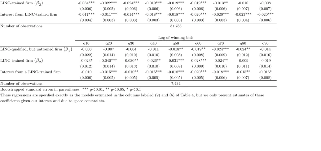
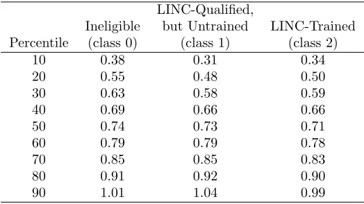
hold not only on average, but might be important throughout the bid distribution. As such, in Table
5, we complement the bid regressions presented above by providing a portion of some quantile bid 13
Table 5: Quantile Bid Regression Results
Log of bids
Variable q10 q20 q30 q40 q50 q60 q70 q80 q90
LINC-qualified, but untrained firm(β1) -0.005 0.001 -0.001 -0.004 -0.002 -0.008 -0.001 0.002 0.020
(0.006) (0.006) (0.005) (0.007) (0.006) (0.009) (0.008) (0.009) (0.015)
LINC-trained firm(β2) -0.034*** -0.022*** -0.024*** -0.019*** -0.019*** -0.019*** -0.013** -0.010 -0.008
(0.006) (0.005) (0.006) (0.006) (0.006) (0.006) (0.006) (0.007) (0.007)
Interest from LINC-trained firm -0.017*** -0.011*** -0.014*** -0.018*** -0.018*** -0.020*** -0.020*** -0.023*** -0.020***
(0.004) (0.003) (0.003) (0.003) (0.003) (0.003) (0.003) (0.004) (0.006)
Number of observations 31,783
Log of winning bids
q10 q20 q30 q40 q50 q60 q70 q80 q90
LINC-qualified, but untrained firm(β1) -0.003 -0.007 -0.004 -0.011 -0.018** -0.019** -0.024*** -0.024** -0.014
(0.022) (0.014) (0.010) (0.010) (0.008) (0.008) (0.009) (0.012) (0.016)
LINC-trained firm(β2) -0.023* -0.040*** -0.030** -0.026** -0.031*** -0.028*** -0.024** -0.009 -0.019
(0.012) (0.014) (0.013) (0.010) (0.008) (0.009) (0.010) (0.011) (0.014)
Interest from a LINC-trained firm -0.010 -0.015*** -0.010** -0.015*** -0.018*** -0.020*** -0.018*** -0.015** -0.015*
(0.006) (0.005) (0.005) (0.005) (0.005) (0.005) (0.006) (0.007) (0.008)
Number of observations 7,434
Bootstrapped standard errors in parentheses. *** p<0.01, ** p<0.05, * p<0.1
These regressions are specified exactly as the models estimated in the columns labeled (2) and (6) of Table 4, but we only present estimates of these coefficients given our interest and due to space constraints.
regression results for the models estimated in the columns labeled (2) and (6) of Table 4. We limit
presentation to these two models as conveying estimates at each decile requires more space. As such, we
also limit our presentation to the estimates of our primary coefficients of interest (those corresponding
to the LINC-related variables in the top three rows of our bid regression table). Nonetheless, the
models estimated are specified exactly as they were in columns (2) and (6) of Table 4 in the sense that
all of the other covariates and fixed effects were included in the estimation. Table 5 has two parts: the
top set of estimates concerns the log of all bids as the response variable, while the bottom relate to
the log of only winning bids. The results discussed above concerning the bidding behavior of
LINC-qualified firms hold throughout much of the distribution. If a firm is LINC-LINC-qualified, but untrained, its
bidding behavior is never statistically different from the ineligible firms; however, LINC-trained firms
behave more aggressively by submitting bids that are 1.3–3.4% lower than the other firms throughout
the first seven deciles of all tendered bids. The indirect competition effect is statistically significant
for every quantile presented. The magnitude of these coefficients is also consistent with the
least-squares estimate. The results concerning winning bids also appear to hold not just at the mean bid,
but throughout much of the distribution. Unlike the least-squares regressions, the winning bids from
LINC-qualified, but untrained firms are statistically different from (lower than) ineligible-firm winning
bids for the median through the 80th percentile. As such, there is some resemblance in the winning
bids from untrained and trained firms for this part of the winning bid distribution. Still, winning bids
from LINC-trained firms are significantly lower than those from ineligible firms for seven of the nine
deciles and the indirect competition effect is significant for all but the lowest decile of the winning bid
distribution.
One may also wonder whether LINC training (or the qualification of LINC-eligibility) might be
affecting bidding behavior through other important channels. For example, the results in Table 4
suggest that many covariates, as we discussed above, might be important in driving the bidding
decisions of firms. Backlog or capacity constraints as well as distance to a project location and strength
of the competition have all been salient issues in important empirical papers concerning auctions; as
Table 6: Investigating other Possible Asymmetries through Bid Regressions
Variable Log of bids Log of winning bids
(1) (2) (3) (4) (5) (6)
LINC-qualified, but untrained firm (β1) -0.001 0.025 0.021 -0.013 0.028 0.008
(0.007) (0.017) (0.016) (0.012) (0.028) (0.025) LINC-trained firm (β2) -0.016** -0.033** -0.046** -0.039*** -0.038 -0.056**
(0.007) (0.015) (0.019) (0.012) (0.025) (0.024) Interest from LINC-trained firm -0.016*** -0.016*** -0.016*** -0.014*** -0.014*** -0.014***
(0.004) (0.004) (0.004) (0.005) (0.005) (0.005) Bidder’s capacity utilized 0.030*** 0.030*** 0.030*** 0.010 0.014* 0.014* (0.005) (0.005) (0.005) (0.009) (0.008) (0.008) Bidder’s capacity utilized× 0.019 0.029
LINC-qualified, but untrained firm (β1) (0.021) (0.032)
Bidder’s capacity utilized× -0.006 0.063* LINC-trained firm (β2) (0.020) (0.037)
Log of bidder’s distance to the project location 0.015*** 0.015*** 0.015*** 0.006*** 0.006*** 0.006*** (0.001) (0.001) (0.001) (0.002) (0.002) (0.002) Log of bidder’s distance to the project location× -0.006 -0.009
LINC-qualified, but untrained firm (β1) (0.004) (0.007) Log of bidder’s distance to the project location× 0.004 0.003 LINC-trained firm (β2) (0.003) (0.006)
Average rivals’ winning-to-plan holder ratio -0.063* -0.063* -0.064* -0.204*** -0.202*** -0.205*** (0.035) (0.035) (0.035) (0.039) (0.039) (0.040) Average rivals’ winning-to-plan holder ratio× -0.132 -0.109 LINC-qualified, but untrained firm (β1) (0.101) (0.162)
Average rivals’ winning-to-plan holder ratio× 0.205 0.221
LINC-trained firm (β2) (0.132) (0.157)
Material shares Yes Yes Yes Yes Yes Yes
Time effects Yes Yes Yes Yes Yes Yes
Project division effects Yes Yes Yes Yes Yes Yes Number of observations 31,783 31,783 31,783 7,434 7,434 7,434
R2 0.984 0.984 0.984 0.989 0.989 0.989
Clustered (by auction) robust standard errors in parentheses. *** p<0.01, ** p<0.05, * p<0.1
These regressions expand the models presented in the columns labeled (2) and (6) of Table 4 by adding interaction terms.
Silva et al. [2008], as well as Bajari et al. [2014]. We explore these possible channels as ways in which
firms might behave differently given their classification by considering other regression models in Table
6. The table is again partitioned by all bids (the first three columns of estimates) and winning bids
(the last three columns). All of the models estimated include all covariates presented in the columns
labeled (2) and (6) of Table 4 but, due to space constraints we only present coefficient estimates for
our variables of interest and the relevant terms for the newly-considered cases. First, note that the
significance of the LINC-trained dummy variable holds in all expanded models except for the case of
winning bids when we consider asymmetric responses to distance (though the magnitude of the effect
is larger than the results from Table 4, thep-value is 0.13). Second, the results concerning the indirect
The estimates in columns (1) and (4) of Table 6 consider interactions between the bidder’s capacity
utilized and its LINC status. In short, firms eligible for the LINC program who are untrained behave
no differently when it comes to capacity utilized than ineligible firms. Once a firm undergoes LINC
training, behavior on average does not change but there is some evidence (significant at the 10%
level) that LINC-trained winners react to their capacity utilized in a statistically different way from
ineligible firms (though not from LINC-qualified, but untrained firms). In columns (2) and (5), we
consider whether the bids of LINC-qualified firms might be different from ineligible firms based on how
close the firm is to the project site. Again, there is no difference on average in the behavior of qualified
firms compared to ineligible firms, and this does not change once the firm completes LINC training.
Lastly, in columns (3) and (6), we investigate whether these firms might respond differently to the
perceived competitiveness of their rival firms. We consider interactions between our LINC-qualified
dummy variables with the average of their rivals’ winning-to-plan holder ratio. The interactions are
never significant—suggesting response to rivals’ success, though important on average, does not differ
from ineligible firms, whether the LINC-qualified firm is trained or not. These potential explanations
involved asymmetries that could be considered using our observed data. Since there was little evidence
to support them, we consider an alternative later by constructing a structural approach. It is built on
the idea that perhaps the LINC-trained firms bid differently because the program affected something
we cannot observe directly in the data, such as the firms’ cost structure.
A concern one might have with the bid regressions presented thus far is selection bias. As shown
above (Table 2), the decision to participate in LINC is non-random. Moreover, being LINC-qualified
seems to affect entry behavior at auctions (Table 3). If LINC training is allowing firms to identify
contracts that are most appropriate once the plans are held, then the bids observed are non-random.
For example, we as econometricians do not see bids from LINC-trained firms on contracts that they
decided were not worth their time pursuing. We address these concerns using two Heckman-based
corrections. First, we estimate the probability of participating in the LINC training program by using
propensity scores derived from the probit models presented in Table 2. This score will be zero for
but untrained firms.14 This score variable introduces a new variable that we have not included in our
bid regressions, but that will be related to whether a bid is submitted on a contract given a firm holds
plans.15 We use this propensity score along with auction-specific covariates to estimate the probability of a given firm tendering a bid at a certain auction. This constitutes our selection approach, which is
then used in the second-stage bid regressions after evaluating the inverse-Mills ratio at the respective
covariate vector.
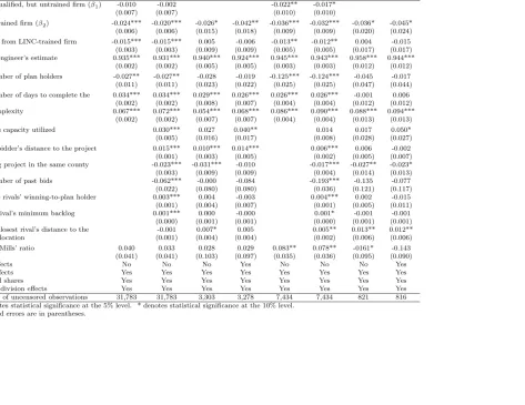
We replicate the models presented in Table 4 following the sample selection procedure discussed
and present corresponding estimates in Table 7. The coefficient on the inverse-Mills ratio is statistically
different from zero in three of the models, all involving winning bids, suggesting sample selectivity is
not overwhelming our estimates.16 Comparing the results here to those presented in Table 4 shows
two things: first, the coefficients of the majority of the covariates we included are largely unchanged;
second, the primary coefficient of interest which measures the effect of LINC training strengthens—
statistical significance of LINC training is achieved in all models now and the magnitude of this effect
is larger in absolute value in nearly ever case. Lastly, the indirect competition effect continues to
generate more aggressive bidding and more aggressive winning bids for nearly all the models.
Lastly, while our focus has been on the awarding of procurement contracts, readers may wonder
whether post-winning behavior either differs across the classes of bidders or somehow cancels the
savings generated at the awarding stage. Taking an extreme position, perhaps LINC graduates have
somehow learned to submit skewed or deceptive bids for a project knowing that they will be able to
renegotiate a higher payment after winning the contract. Such concerns were the basis of Bajari et al.
[2014], in which the authors focused on the prevalence of renegotiation and post-awarding adaptation.
To evaluate this, we obtained data on the final payments made to firms for contracts completed during 14
Two related comments: first, since the LINC program began in 2001, the propensity score of every firm is zero before the inaugural training session; second, since LINC training is not available every month, we use the yearly average for months in which training was not available, which ensures the probability is updated throughout the sample.
15
In models where we consider the log of winning bids, we use a propensity score derived from a probit in which the past winning-to-bidding ratio was used. We felt these were the natural results to present given they represent the underlying selection process we’re trying to address.
16
Table 7: Bid Regression Results with Heckman Approach
Variable Log of bids Log of winning bids
Full sample LINC qualified Full sample LINC qualified
(1) (2) (3) (4) (5) (6) (7) (8)
LINC-qualified, but untrained firm (β1) -0.010 -0.002 -0.022** -0.017*
(0.007) (0.007) (0.010) (0.010)
LINC-trained firm (β2) -0.024*** -0.020*** -0.026* -0.042** -0.036*** -0.032*** -0.036* -0.045*
(0.006) (0.006) (0.015) (0.018) (0.009) (0.009) (0.020) (0.024)
Interest from LINC-trained firm -0.015*** -0.015*** 0.005 -0.006 -0.013** -0.012** 0.004 -0.015
(0.003) (0.003) (0.009) (0.009) (0.005) (0.005) (0.017) (0.017)
Log of engineer’s estimate 0.935*** 0.931*** 0.940*** 0.924*** 0.945*** 0.943*** 0.958*** 0.944***
(0.002) (0.002) (0.005) (0.005) (0.003) (0.003) (0.012) (0.012)
Log number of plan holders -0.027** -0.027** -0.028 -0.019 -0.125*** -0.124*** -0.045 -0.017
(0.011) (0.011) (0.023) (0.022) (0.025) (0.025) (0.047) (0.044)
Log number of days to complete the 0.034*** 0.034*** 0.029*** 0.026*** 0.026*** 0.026*** -0.001 0.006
project (0.002) (0.002) (0.008) (0.007) (0.004) (0.004) (0.012) (0.012)
Log complexity 0.067*** 0.072*** 0.054*** 0.068*** 0.086*** 0.090*** 0.088*** 0.094***
(0.002) (0.002) (0.007) (0.007) (0.004) (0.004) (0.013) (0.013)
Bidder’s capacity utilized 0.030*** 0.027 0.040** 0.014 0.017 0.050*
(0.005) (0.016) (0.017) (0.008) (0.028) (0.027)
Log of bidder’s distance to the project 0.015*** 0.010*** 0.014*** 0.006*** 0.006 -0.002
location (0.001) (0.003) (0.005) (0.002) (0.005) (0.007)
Ongoing project in the same county -0.023*** -0.031*** -0.010 -0.017*** -0.027** -0.023*
(0.003) (0.009) (0.009) (0.004) (0.014) (0.013)
Log number of past bids -0.062*** -0.000 -0.084 -0.193*** -0.135 -0.077
(0.022) (0.080) (0.080) (0.036) (0.121) (0.117)
Average rivals’ winning-to-plan holder 0.003*** 0.004 -0.003 0.004*** 0.002 -0.015
ratio (0.001) (0.004) (0.007) (0.001) (0.005) (0.011)
Log of rival’s minimum backlog 0.001*** 0.000 -0.000 0.001* -0.001 -0.001
(0.000) (0.001) (0.001) (0.000) (0.001) (0.001)
Log of closest rival’s distance to the -0.001 0.007* 0.005 0.005** 0.013** 0.012**
project location (0.001) (0.004) (0.004) (0.002) (0.006) (0.006)
Inverse-Mills’ ratio 0.040 0.033 0.028 0.029 0.083** 0.078** -0161* -0.143
(0.041) (0.041) (0.103) (0.097) (0.035) (0.036) (0.095) (0.090)
Firm effects No No No Yes No No No Yes
Time effects Yes Yes Yes Yes Yes Yes Yes Yes
Material shares Yes Yes Yes Yes Yes Yes Yes Yes
Project division effects Yes Yes Yes Yes Yes Yes Yes Yes
Number of uncensored observations 31,783 31,783 3,303 3,278 7,434 7,434 821 816
** denotes statistical significance at the 5% level. * denotes statistical significance at the 10% level. Standard errors are in parentheses.
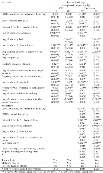
the years of our data sample.17 In Table 8, we provide estimates from four models (two based on
least-squares and two which address sample-selection concerns in the way we discussed above) in which our
dependent variable is now the final payment made to the winning bidder, post any renegotiation and/or
adjustments to the projects. The estimates in columns (1) and (3) condition on the engineer’s initial
estimate of the project while the estimates in columns (2) and (4) consider the winning bid. When the
engineer’s estimate is considered, the estimated coefficients for our direct and indirect LINC-related
effects are nearly identical to those we obtained when the winning bid was used as a dependent variable.
Thus, cost savings implied by the awarding stage are actually realized when the state writes its final
check to the firm who completes the task. LINC-trained bidders are paid 3% less on average and the
indirect competition effect generates savings of over 2%. When the winning bid is considered on the
right-hand side, there is no significant effect of being a LINC-trained firm and no indirect competition
effect. This is reassuring as it suggests that behavior in the post-awarding stage is unrelated to
LINC-training and does not differ across our classes of bidders. Having considered this, we feel confident in
saying that LINC graduates are not somehow manipulating the system in a way that wipes out any
suggested savings the state receives from the auction. Moreover, renegotiation and/or adjustments
needed after the contract has been awarded appear to be independent of which class bidders belong
to.
In the introduction, we noted that operation of the LINC program costs the state about $200,000
per year. Using our estimates from model (6) of Table 4 (analogously, model (6) from Table 8 has nearly
the same predictions) we can provide an estimate of the benefits the LINC program has generated.
Specifically, we look in the data and identify which auctions were won by either (i) a LINC-trained
firm for a project multiple LINC-trained firms were interested in, (ii) a LINC-trained firm in which
the winning firm was the only LINC-trained firm that showed interest in the project, or (iii) a
non-LINC-trained firm who won a contract that attracted the interest of a non-LINC-trained firm. We use
the coefficient point estimates from the LINC-trained dummy and the indirect competition variable to 17
Table 8: Bid Regression Results for Final Payments
Variable Log of final pay (completed projects only) OLS Heckman (1) (2) (3) (4) LINC-qualified, but untrained firm (β1) -0.003 -0.006 -0.007 -0.008
(0.014) (0.008) (0.015) (0.010) LINC-trained firm (β2) -0.030** 0.002 -0.031** 0.001
(0.012) (0.008) (0.012) (0.008) Interest from LINC-trained firm -0.025*** -0.004 -0.023*** -0.003
(0.007) (0.005) (0.007) (0.005) Log of engineer’s estimate 0.935*** 0.933***
(0.006) (0.005)
Log of winning bid 0.994*** 0.993*** (0.004) (0.003) Log number of plan holders -0.077*** -0.014** -0.104*** -0.029
(0.010) (0.006) (0.033) (0.021) Log number of days to complete the 0.045*** 0.012** 0.045*** 0.012*** project (0.008) (0.005) (0.007) (0.004) Log complexity 0.083*** -0.001 0.085*** 0.000
(0.008) (0.006) (0.007) (0.004) Bidder’s capacity utilized 0.024* 0.005 0.024* 0.005
(0.013) (0.008) (0.013) (0.008) Log of bidder’s distance to the project 0.000 -0.004* 0.000 -0.004** location (0.003) (0.002) (0.003) (0.002) Ongoing project in the same county -0.015** 0.002 -0.015** 0.002
(0.007) (0.004) (0.007) (0.004) Log number of past bids -0.200*** 0.032 -0.196*** 0.034
(0.066) (0.044) (0.061) (0.039) Average rivals’ winning-to-plan holder -0.000 -0.004** -0.000 -0.004*** ratio (0.002) (0.002) (0.002) (0.001) Log of rivals’ minimum backlog 0.001 -0.000 0.001 -0.000
(0.000) (0.000) (0.000) (0.000) Log of closest rival’s distance to the 0.000 -0.004** 0.001 -0.004** project location (0.003) (0.002) (0.003) (0.002)
Selection
LINC-qualified, but untrained firm (β1) -0.149*** -0.149*** (0.055) (0.055) LINC-trained firm (β2) 0.555 0.555
(0.373) (0.373) Interest from LINC trained firm 0.078*** 0.078***
(0.024) (0.024) Log of engineering estimate -0.064*** -0.064***
(0.014) (0.014) Log number of plan holders -1.013*** -1.013***
(0.033) (0.033) Log number of days to complete the -0.002 -0.002
project (0.021) (0.021)
Log complexity 0.062*** 0.062*** (0.019) (0.019) LINC participation probability – based -0.603 -0.603 on past winning-to-bidding ratio (0.371) (0.371)
λ 0.039 0.021
recompute how much more expensive the auctions would have been had the respective firm not been
LINC trained. Aggregating the savings across the three types of winning scenarios noted implies cost
savings of over $21 million per year—this amounts to 1.49% of the total value of the engineer’s estimates
for these contracts and 1.55% of the total value of the actual winning bids for these contracts.18 The
negligible cost to TxDOT of running the LINC program pales in comparison to the funds saved and
suggests large government savings. Another way to quantify the effect of the LINC program involves
calculating the number of additional plan holders or bidders per auction that would be required to
induce the same cost savings. Again, using the estimates from model (6) of Table 4 suggests that
TxDOT would need to have, on average, an additional 0.95 plan holders or 0.56 bidders per auction
to yield the same cost savings.
Our work here has measured the effects of LINC on participation, behavior, and success in TxDOT
procurement contracting. However, the LINC program may imply changes to the cost structure of
graduate firms. For example, perhaps their costs are improving which is allowing them to be more
successful. In the same vein, it would be interesting to look at whether the efficiency of the procurement
auctions has improved as a result of the LINC training program. Of course, analyzing bidding behavior
is reasonably straightforward as bids are observed directly, but shedding light on these other issues
involves understanding the (unobserved) cost structures of the firms. To investigate these questions
involving firms’ costs and the efficiency of the auctions, we construct a structural model of bidding
behavior in the next section and present insight from estimating the latent cost distributions in the
section that follows.
4
Structural Model of Bidding
In this section, we investigate further the change in observed bidding patterns by appealing to a
theoretical model in which we allow for asymmetric bidders.19 Note that we do not impose such an
18
We compute a 95% confidence interval for these predictions by considering the coefficient estimates plus and minus the appropriate number of standard deviations and then re-predicting cost savings. Such an exercise puts the cost savings in the range of [$7.1 million,$41.7 million].
19
asymmetry in our analysis, but rather, allow for the possibility in our estimation strategy which is
nonparametric and, thus, data-driven. We organize this section as follows. In the first subsection,
we describe the underlying model. In the second subsection, we discuss practical issues including the
pooling of many types of heterogeneous auctions in which the composition of bidders differs in our
empirical work.
4.1
Asymmetric Procurement Model
Consider TxDOT would like to complete an indivisible task at the lowest possible cost. Tenders are
invited fromn(≥2) bidders (firms) and are opened only once a submission deadline has passed. The
contract is awarded to the lowest bidder, who wins the right to perform the task. TxDOT pays the
winning firm its bid on completion of a contract. Assume that there is no price ceiling—a maximum
acceptable bid that has been imposed by the buyer20
Assume bidders (firms) are risk neutral and belong to one of three classes.21 Specifically, we refer
to class 0 bidders as the ineligible/non-LINC bidders, to class 1 bidders as the LINC-eligible, but
untrained bidders or the never trained bidders, and to class 2 bidders as the LINC graduates or the
LINC-trained firms. Again, class 1 includes firms who are eligible and choose to never undergo LINC
training and firms that eventually partake in the LINC program, but are observed before doing so.22 Thus, a given firm may be a class 1 bidder in some auctions that took place early, chronologically
speaking, and then, after completing the LINC program, be a class 2 bidder in later auctions. In such
instances, the pre-training bids are considered to be from a class 1 bidder, while the post-graduation
means the prime contractor (bidder) can realize cost savings (or extract potential rents) by knowing when to use various suppliers who might specialize in a smaller subset of tasks. In addition, part of the training involves learning project-management techniques.
20
This is reasonable as, in our data, such a value is never imposed nor is a contract ever not awarded due to bidding behavior, even though there are instances in which the winning bid for a contract exceeds an engineer’s estimate of the cost to complete a given project. There are a small number of instances in which TxDOT cancels a project and then either redesigns it or combines it with other outstanding work.
21
We are careful to refer to bidders as belonging to one of three classes and not as being of one of threetypes to prevent confusion with theoretical research concerning auctions. In that literature, a bidder of a certain type means a bidder having a specific cost value, regardless of which class she belongs to.
22