Redundant feature selection using permutation methods

http://wrap.warwick.ac.uk

Taylor, P., Griffiths, Nathan and Bhalerao, Abhir (2015) Redundant feature selection using permutation methods. In: AutoML workshop @ ICML'15, Lille, France, 11 Jul 2015

Permanent WRAP url:

http://wrap.warwick.ac.uk/72876

Copyright and reuse:

The Warwick Research Archive Portal (WRAP) makes this work by researchers of the University of Warwick available open access under the following conditions. Copyright © and all moral rights to the version of the paper presented here belong to the individual author(s) and/or other copyright owners. To the extent reasonable and practicable the material made available in WRAP has been checked for eligibility before being made available.

Copies of full items can be used for personal research or study, educational, or not-for profit purposes without prior permission or charge. Provided that the authors, title and full bibliographic details are credited, a hyperlink and/or URL is given for the original metadata page and the content is not changed in any way.

A note on versions:

Redundant Feature Selection using Permutation Methods

Phillip Taylor [email protected]

Nathan Griffiths [email protected]

Abhir Bhalerao [email protected]

The University of Warwick, CV4 7AL, UK

Abstract

Automatic feature selection aims to select the features with highest performance when used in a classifier. One popular measure for estimating feature relevancy and redundancy is Mutual Information (MI), although it is biased toward features with multiple values. Permutation methods have been successfully applied in normalizing for numerous biases including that of MI; however they are computationally expensive and complete redundancy computation is infeasible. In this paper, we introduce a measure that can be used to approximate allm2_{redundancies betweenmfeatures, while performing onlympermutation} methods for their relevancies. We then show using simulated data that this permutation redundancy measure holds similar properties to normalized MI and apply it in selecting features from example datasets using minimal Redundancy Maximal Relevancy (mRMR).

1. Introduction

Taylor Griffiths Bhalerao

2. Background

The permutation method is a statistical test that can be used to assign a significance to a correlation between two variables such asM I(x, y), or to normalize it for biases (Good,2000;

Hapfelmeier and Ulm, 2013). It operates by computing the correlation statistic for several different permutations (1000 in this paper) of the variables. Permuting either variable gives the same permutation distribution, and it is computationally more efficient to permute the class labels when computing relevancies rather than each individual feature.

The significance, orp-value, is the proportion of the permutation distribution that is at least as large asM I(x, y). Rather than compute ap-value,Wang et al.(2009) assume that the distribution is normally distributed and use the standard score of M I(x, y),

ZMI(x,y) =

M I(x, y)− {y0 ∈Ψ(y) :M I(x, y0)}µ {y0 _{∈Ψ(y) :M I(x, y}0_)}

σ

, (1)

where Ψ(y) is the set of computed permutations ofy, andµand σ represent the mean and standard deviation. Radivojac et al.(2004), useZM I to rank features withp-values below a threshold. The other features are ranked by their p-value and below those ranked by ZM I. A popular filter for feature selection introduced by Peng et al. (2005) is mRMR. In general, mRMR aims to maximize the difference or ratio between the mean relevancy, Rel(·), and redundancy, Red(·), of selected features (Herman et al.,2013). In this paper we use a forward greedy search to select the feature that satisfies,

max

x∈X\S Rel(xi, y)− 1

|S∪ {x}|2

X

xi,xj∈S∪{x}

Red(xi, xj), (2)

where X ={x0, x1, . . . , xn} is the complete set of input features, y is the target variable, and S⊂X is the set of currently selected features. Where bothRel(·) and Red(·) is given by MI, it is referred to asM ImRM R in this paper.

3. A redundant permutation feature selector

UsingZM I as a measure of both relevancy and redundancy in mRMR is prohibitive for even small feature sets, and has a worst case of m+m2 permutation methods when computing a full ranking. Therefore, we propose a redundancy metric that is calculated directly from the permutation distributions produced in computing the relevancies, requiring exactly m permutation methods to compute all redundancies. Specifically, we suggest that the similarity of the relevancy permutation distributions be used to estimate redundancy.

If two binary features, x1 and x2, are mutually redundant and M I(x1, x2)≈1, then we can say that their relevancies are similar;M I(x1, y)≈M I(x2, y) for any targety. A corol-lary of this is that dissimilar relevancies,M I(x1, y)6≈M I(x2, y), imply that the features are not redundant;M I(x1, x2)6≈1. Unfortunately, similar relevancies,M I(x1, y)≈M I(x2, y), do not guarantee that the features are redundant, and there may be unrelated features with similar relevancies. Knowledge of relevancies does, however, provide some insight into the feature redundancy relationship. For instance, if the two relevancies, M I(x1, y) and M I(x2, y), are similar then the features are more likely to be redundant than if the relevan-cies are very different. Furthermore, if it is known that the features have similar relevanrelevan-cies

with many different targets, the likelihood of their redundancy is increased. This is the basis of the proposed permutation redundancy measure.

The permutation redundancy measure is computed by performing the permutation method for several features simultaneously, permuting only the target at each iteration. For a given permutation, y0, the permutation correlations, M I(xi, y0) are recorded for all features xi ∈ X. Imagine that for all computed permutations of y, Ψ(y), the permutation correlations for features x1 and x2 are similar, i.e. M I(x1, y0)≈M I(x2, y0)∀y0 ∈Ψ(y). In this case it is reasonable to conclude that x1 andx2 are related and redundant features. If they were not related, some proportion of the permutation correlations would be dissimilar. Permutation distributions are not directly comparable by a measure such as mean abso-lute difference, because the permutation correlations share the same bias found in MI and increase with the dimensionality of a feature. Instead, to successfully compare distributions of different ranges, we use Pearson’s Correlation Coefficient,

P CM I(x1, x2, y) =P CC(M I(x1, y0), M I(x2, y0) :∀y0 ∈Ψ(y)). (3)

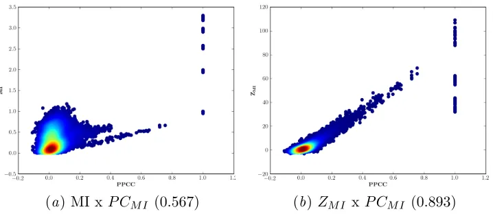
Simulated data is used to show the relationship between MI,ZM I andP CM I. The data is simulated by generating a uniform binary string of 100 independent samples which is taken to be the target, y. A total of 125 features are then generated by copying this target and changing their sample values randomly to decrease their relationship withy and their cardinalities to increase their entropy and bias their MI with other features. The features are separated into five sets of 25, each of which has a different percentage of the sample values altered. Specifically, the percentages of changed samples are 5%, 10%, 20%, 30%, 40%; producing features varying in levels of relevancy and redundancy. Each set of 25 features with the same number of value changes is split once more into 5 sub-sets. In the first subset, the features are kept the same and remain binary. In the second, each of the feature values are divided uniformly at random into two, creating features of cardinality 4. The third subset has each of the feature values divided into three, while the fourth and fifth subsets have features of cardinality 8 and 10 respectively. This creates a simulated dataset with 5 features for each value change and value split combination, totalling 125 features.

Taylor Griffiths Bhalerao

(a) MI xP CM I (0.567) (b) ZM I x P CM I (0.893)

Figure 1: Scatter plots of MI (a) and ZM I (b) againstP CM I. Lighter red points indicate higher density regions. The correlations of the measures are shown in braces.

4. Evaluation

To evaluate theM ImRM RandP mRM Rfeature selection methods, we used the Arrhyth-mia, Chess, Congress, Credit, Fertility, Madelon, Musk 1, Parkinsons, Promoters, Soybean (small), Soybean (large), Spambase, Splice, TR11, TR12, TR21, TR23, Vehicles, Wine, and Yeast that are available in the UCI1 _{and Tuned IT}2 _{repositories. These datasets} were chosen because of their range in size and features, as well as their use in previous feature selection literature (Herman et al.,2013). All samples with missing values were first removed from the dataset, before numeric or real valued features were discretized using the minimum descriptive length method (Fayyad and Irani,1993). At this point, features with only one discrete value were discarded as they contain no information. This is so features can be generated from existing ones, while changing their sample values to worsen their predictive performance and increasing their dimensionality to bias MI.

From each dataset, 5 new datasets were generated by copying original features and increasing their dimensionalities. In all cases, before increasing the dimensionality of a feature, 5% of the values were changed to worsen their predictive abilities. The target variable was not copied or altered in any of the new datasets. The 5 datasets, referred to as {1}, {1,2}, {1,2,3}, {1,2,3,4}, and {1,2,3,4,5}, had different numbers of features added to the original ones with different numbers of splits in their values. Dataset{1} had double the number of features as the original, and the values of each added feature were split once to double its dimensionality. All of the features present in{1}were also in{1,2}, with one extra copy of the original features having two splits in their values to triple their dimensionalities. In each of the subsequent datasets an extra copy was added on top of the previous, with one extra split in values applied. In the fourth, fifth and sixth datasets therefore, there were four, five, and six times as many features as in the original dataset, with dimensionalities multiplied by four, five and six respectively.

For each of the datasets a random subset validation procedure with ten train-test it-erations was performed. In each iteration 50% of the samples were taken uniformly at

1.http://archive.ics.uci.edu/ml, 2. http://tunedit.org/repo/Data/

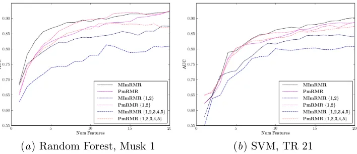
(a) Random Forest, Musk 1 (b) SVM, TR 21

Figure 2: Mean AUCs over ten evaluations with between one and twenty features from Musk 1 (a) and TR 11 (b) datasets and using Random Forest and SVM respectively.

random as training data, from which features were ranked using forward selection with both M ImRM R and P mRM R. To consider relevancy and redundancy of equal impor-tance and for a fair comparison, the relevancies and redundancies in both M ImRM R and P mRM Rwere normalized between 0 and 1, before choosing each feature. Twenty classifiers were then built with increasing numbers of features (between one and twenty) taken from the top of these rankings. The classification algorithms used were Na¨ıve Bayes, Decision Tree, Random Forest, and Support Vector Machine (SVM), which are all available in the WEKA (Witten and Frank,2011) library. The remaining 50% of the samples in each itera-tion were used as testing data to produce a performance measure in the form of a weighted Area Under the ROC (Receiver Operating Characteristic) Curve (AUC). Finally, because features were ranked using the same training samples for both ranking methods, the AUC performances produced during each testing iteration can be compared directly.

For illustration, the mean AUC performances over the ten iterations of the TR 21 and Musk 1 datasets, using the Random Forest and SVM classifiers respectively are shown in Figure2. The plots are representative of using other classifiers with different datasets, and show that AUC decreases as more features with higher dimensionalities present. It also shows that performance decreases less when features are selected usingP mRM Rthan with M ImRM R. In some cases, and mainly with the Decision tree classifier, where AUCs for the original features were close to 1, the mean AUC performance was affected less by the added features than when the AUC for the original dataset was small.

Taylor Griffiths Bhalerao

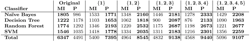
Original {1} {1,2} {1,2,3} {1,2,3,4} {1,2,3,4,5}

Classifier MI P MI P MI P MI P MI P MI P

Na¨ıve Bayes 1805 986 1533 1771 1348 2160 1446 2181 1278 2333 1429 2208

Decision Tree 1222 1178 1103 1653 1062 1818 900 2087 876 2133 1090 1963

Random Forest 1774 1292 1346 2193 1220 2532 1175 2687 1198 2673 1221 2677

SVM 1546 1035 1418 1778 1334 2035 1311 2183 1216 2301 1356 2259

Total 6347 4491 5400 7395 4964 8545 4832 9138 4568 9440 5096 9107

Table 1: Number of times features selected byM ImRM R(MI) outperformed those selected by P mRM R(P), and vice versa, for each classifier over all train-test iterations.

{1} {1,2} {1,2,3} {1,2,3,4} {1,2,3,4,5}

Dataset MI P MI P MI P MI P MI P

Datasets where better 3 15 1 17 1 16 2 16 1 17

Total features 684 848 636 838 609 814 616 825 614 819

Table 2: Number of original features ranked by in top five by M ImRM R (MI) and P mRM R(P) over all train-test iterations.

A good feature ranking method should rank the original features higher than the injected ones, as randomizing values in the copies means that they are worse predictors of the target. The total number of times an original feature was ranked in the top five byM ImRM Rand P mRM Rfor the datasets with extra features are shown in Table2. Detailed results for each dataset are omitted for space reasons, but the number of datasets where one outperformed the other in this task are presented. Overall, as features were copied more and with more splits, fewer original features were ranked in the top five by bothM ImRM RandP mRM R. In the majority of cases, P mRM R outperformed M ImRM R, and M ImRM R was again more affected by increasing the dimensionality of features than wasP mRM R. One notable case where M ImRM R outperformed P mRM R is with the Congress dataset, which is small and simple in structure. In fact, when the top ten or twenty features in the rankings are considered, P mRM RoutperformsM ImRM R less often, withM ImRM R performing better for several smaller datasets including Credit, Fertility, and Soybean (small).

5. Conclusion

This paper investigated redundant feature selection using permutation normalized correla-tions. We showed with simulated data that permutation normalized MI can be estimated accurately by comparing permutation distributions computed from a common target. A nor-malized variant of mRMR was used to successfully select features from example datasets with extra features to increase the difficulty of the selection problem. Our approach can automatically select features and requires no parameters other than the number of permu-tations – which should be as large as is computationally reasonable.

As future work we intend to investigate the relationship between the number of permuta-tions used, and the performance of the features selected using the permutation redundancy measure. We also intend to investigate different feature selection filters with the redundant permutation measure, such as feature clustering (Li et al.,2008).

References

A. Altmann, L. Tolo¸si, O. Sander, and T. Lengauer. Permutation importance: a corrected feature importance measure. Bioinformatics, 26(10):1340–1347, 2010.

S. Chen. Redundant feature selection based on hybrid GA and BPSO. In International Conference on Communication Software and Networks, pages 414–418, 2011.

U. Fayyad and K. Irani. Multi-interval discretization of continuous-valued attributes for classification learning. Machine Learning, 1993.

P. Good. Permutation tests: a practical guide to resampling methods for testing hypotheses, volume 2. Springer New York, 2000.

I. Guyon and A. Elisseeff. An introduction to variable and feature selection. Journal of Machine Learning Research, 3:1157–1182, 2003.

A. Hapfelmeier and K. Ulm. A new variable selection approach using random forests.

Computational Statistics &Data Analysis, 60:50–69, 2013.

G. Herman, B. Zhang, Y. Wang, G. Ye, and F. Chen. Mutual information-based method for selecting informative feature sets. Pattern Recognition, 46(12), 2013.

D. Jensen and P. Cohen. Multiple comparisons in induction algorithms. Machine Learning, 38(3):309–338, 2000.

R. Kohavi and G. John. Wrappers for feature subset selection. Artificial Intelligence, 97 (1-2):273–324, 1997.

G. Li, X. Hu, X. Shen, X. Chen, and Z. Li. A novel unsupervised feature selection method for bioinformatics data sets through feature clustering. InIEEE International Conference on Granular Computing, pages 41–47, 2008.

H. Peng, F. Long, and C. Ding. Feature selection based on mutual information criteria of max-dependency, max-relevance, and min-redundancy. IEEE Transactions on Pattern Analysis and Machine Intelligence, 27(8):1226–1238, 2005.

P. Radivojac, Z. Obradovic, K. Dunker, and S. Vucetic. Feature selection filters based on the permutation test. In European Conference on Machine Learning, pages 334–346. Springer, 2004.

P. Taylor, F. Adamu-Fika, S. Anand, A. Dunoyer, N. Griffiths, and T. Popham. Road type classification through data mining. In Proceedings of the International Conference on Automotive User Interfaces and Interactive Vehicular Applications, pages 233–240, 2012.

Taylor Griffiths Bhalerao

J. Wang, W. Lee, and M. McKeown. A novel segmentation, mutual information network framework for EEG analysis of motor tasks. BioMedical Engineering OnLine, 8(1):1–19, 2009.

I. Witten and E. Frank. Data Mining: Practical Machine Learning Tools and Techniques. Series in Data Management Systems. Morgan Kaufmann, 2011.