Training deep learning models to count based on synthetic data

CREATIVE TECHNOLOGY BACHELOR THESIS REPORT

TEACHING DEEP LEARNING

MODELS TO COUNT BASED ON

SYNTHETIC DATA

van den Brink, G.C. (Corjan) [email protected] s1733826

Supervisor: Dr. Andreas Kamilaris

Abstract

Training deep convolutional neural networks requires a significant amount of data. Solving the

need for real-world training data that is hard and expensive to create, this research project tries

to design both a deep convolutional neural network and a synthetic dataset for training. Using

synthetic data in training solves the need for big real-world datasets. In this training, a

customized deep neural network allows for a more tailored approach to learning and

generalizing the training. The context is a regression problem dealing with counting houses on

satellite images. As a result, this research presents a combined model able to count houses on

images in a real-world testing dataset with an average counting error of 3 for images with a

number of houses in range [0, 38]. The combined model consists of a deep convolutional neural

network and a linear regression model. This research concludes that creating a custom model is

a good, but complicated, way of solving specific counting problems and that the method of

creating synthetic data is very important in arriving at a good solution.

Acknowledgements

This project was supervised by Dr. Andreas Kamilaris, who I’d like to thank for this interesting

and broadening experience into the field of deep learning. His instructions, feedback and

connections to colleagues were important to defining useful experiments. In his patience I was

able to explore and research this area within this project.

I’d like to thank Max Van Vugt as he laid the foundation for this thesis in the preparatory work he

did at the end of his thesis. His work provided a backbone to this project.

Thanks to Ir. Richard Bults as coordinator for the graduation projects inside the Creative

Technology studies at the University of Twente for allowing a smooth application for this project

and his other organising work around the theses this semester.

Thanks to Faiza Bukhsh for being my critical observer and for allowing me to improve my work

Table of Contents

Abstract... 1

Acknowledgements ... 1

Table of Contents ... 2

List of Figures ... 3

Chapter 1 - Introduction ... 4

Chapter 2 – State of the Art... 6

Discussion ... 6

Preliminary conclusion ...10

Chapter 3 - Methods and Techniques ...11

Chapter 4 Ideation ...13

Orientation ...13

Preparatory work ...14

Tinkering ...15

Research ...15

Requirements ...16

Chapter 5 Realisation...18

Baseline model ...18

Custom model ...20

Chapter 6 Evaluation...25

Per model ...25

Project ...32

Chapter 7 – Conclusion ...33

Chapter 8 – Future Work ...35

Appendix 1 - model and training experiments tree ...36

Appendix 2 - data experiments tree ...37

Appendix 3 - VGG baseline network architecture ...38

Appendix 4 - custom template model visualisation ...39

Appendix 5 – result graphs of training and validation on real data per model ...40

List of Figures

Figure 1 Synthetic data version 1 (Max) examples ...14

Figure 2 Validation data examples with added labels (Max) on top ...15

Figure 3 Synthetic data version 2 examples ...19

Chapter 1 - Introduction

In recent years, research in the field of deep learning has advanced enormously. Deep learning

enables training of a neural network or model, which is capable of learning relations in data at a

level that humans can most of the time not attain. Applications of this relatively new technology

are already being implemented in various aspects of daily life. Still, most of these applications

exist based on training with real-world datasets. To train a deep learning model or deep neural

network well, data should be provided in big quantities [1], [2]. However, in a lot of cases, this

data does not exist at all or in big enough quantities in the real world [3]. So, it must be gathered

and labelled, which is very labour-intensive, error-prone and therefore costly. Especially in the

case of counting problems (i.e. problems where a model learns to count a certain object based

on its occurrence in the provided training data) this type of data is hard to come by and very

challenging and time-consuming to create.

A solution to this is to train the deep neural networks on synthetic data that replaces the needed

real-world training dataset. This synthetic data should be representative of the type of data that

would be used in training with real-world data [4]. The training should be generalized by the

network to be applicable in the real world [1], [4]. This solution provides the ability to train the

deep neural networks also in situations where real data is hard to come by and in general,

should simplify training these networks by not requiring as much real data for the training.

In this report, the use of synthetic (visual) data in the training of a deep convolutional neural

network in solving regression problem dealing with counting will be explored. The application of

this technology in the context of this research is very novel and shows great promise. By

exploring this problem and trying to find a solution that is based on other recent findings and

ideas this should be beneficial to future research in this area. The solution should present a

working deep convolutional neural network, trained on designed synthetic data. The process of

designing both the model and the data, should lead to an answer to the following research

question. This answer should define or help define a method for creating synthetic data together

with a deep convolutional neural network that uses this data in its training.

In what way should a deep convolutional neural network be designed to train on synthetic data

in a regression problem dealing with counting while being able to generalize its knowledge well

Two different aspects are identified in this main question. First, designing a deep convolutional

neural network that will train to generalize well on instances of real-world data. Second,

designing synthetic data for training the model on. An important aspect of answering the

research question is connected to designing and testing the influence of different iterations of

synthetic data. Both the neural network and the synthetic data will be investigated throughout

this thesis by doing experiments based in a defined context. The context of this assignment will

be to count houses on satellite images of suburbs in Tanzania. This was inspired by the Open

AI Tanzania challenge from werobotics1_.

This thesis builds on some work done by Max van Vugt [5]. He investigated the use of deep

learning with synthetic data in the context of a categorisation problem dealing with forest fires

and started preparing work in the context of this project. By preparing the validation data, a

simple synthetic dataset and investigating on the regression problem by training some models

from literature, he set the first steps in this project.

From his work, he concluded that creating synthetic images to train deep convolutional neural

networks is a method that needs lots of tailoring before being applicable to different sort of

problems. Therefore, it would be difficult to apply the method that worked well in solving his

classification problem to this new regression problem. Additionally, the models he used seemed

to not be able to learn and predict properly on his data. Throughout this project parts of his

research are reused and improved upon.

Chapter 2 – State of the Art

Discussion

In the process of answering the introduced research question, the first step is doing literature

research. The exact process of doing research will be explained in chapter 3 and 4. This

state-of-the-art chapter is a review of the most important literature background for this project. In this

review, first, the terminology in the question is addressed. This entails the subjects of deep

learning, convolutional neural networks, counting problems, and synthetic data. These are

explored by looking at some fundamental and early research in the field of deep learning. These

more fundamental papers are useful as they usually define what the ideas or intentions behind

the specific concepts are, which is useful to keep in mind during the project. This fundamental

research opens two paths, that can be taken to find a solution for the counting problem faced.

Either using existing pre-trained networks or using a more custom self-built network are

discussed to show both these paths. Surrounding research provides insights for making design

choices when this second option is considered. Building an understanding of what the field is

about and how designs for networks are justified will lead to a preliminary conclusion to the

central question.

Advancements in deep learning

For understanding the general terminology in the research field of deep learning, a review paper

of LeCun, Bengio, and Hinton (2015) provides a useful summary. They describe the

advancements in this area of machine learning in a simple way, enabling the basic

understanding of some key topics. Their focus is on the method of supervised learning as most

current research is based on this type of training. In supervised learning, the deep neural

networks train to learn labelled representations.

For a long time, the field of machine learning focused on trying to find optimal feature extractors

to detect and recognize patterns in data. However, deep learning is able to find these on its own

and has now been adopted in most of the image and language recognition areas as it simplifies

the task of extracting interesting features in data [6].

ConvNets

Convolutional neural networks (for short ConvNets or CNN’s) are a variant of neural networks

which include convolutional layers. ConvNets were another big step forward in the field of deep

every neuron in the next layer (these are called fully connected layers). Convolutional layers are

especially useful for feature extraction. They ‘look’ at a local area of the data to find something that LeCun et al. (2015) call “motifs”. These motifs are found by a “filter bank” which creates a “feature map” showing the specific motifs. The filter banks vary for every feature map and in this

way different motifs can be detected. The idea is that by pooling these convolutional layers,

similar features get merged and a more robust recognition system is created. Stacking the

convolutional and pooling operations on top of each other several times creates a recognition

system similar to the biological vision system [7]. ConvNets can recognize complex

representations by distinguishing basic motifs and combining these into more complex features.

In the context of this review, these complex representations are objects in an image.

Counting with ConvNets

In a paper by Seguì, Pujol, and Vitria (2015) a counting problem is combined with convolutional

neural networks. The sort of counting problem explored is a counting problem that falls under

‘weakly’ supervised learning. This is claimed to be the first problem where only the number of

countable objects is given. Other researches have investigated the problem of counting objects,

but in a different way; first segmenting the data and then counting these segments [9], [10]. The

hypothesis in this paper is, that using ConvNets the network learns what it is counting.

Therefore, it should be able to make accurate predictions on the count of specific objects based

on very simple labelling.

This hypothesis is tested by counting even numbers in random visualizations containing both

odd and even numbers from the MNIST dataset for written digits [11]. To test in different

contexts, the paper also deals with the counting problem of pedestrians on camera images; a

specific problem that multiple researchers have paid attention to [12].

The research of Seguì et al. concludes that the task of counting even numbers in pictures where

both odd and even numbers are present enables the trained network to be able to distinguish

between odd and even as well as being able to categorize individual digits. This last task is a

“more different” task than the original counting problem. It shows that counting problems using

ConvNets can be a very powerful training setup.

Additionally, Seguì et al. test to see where the model detects the features and from this, it

shows that ConvNets trained in a counting problem can locate the features of interest. This

Synthetic data

Seguì et al. (2015) use synthetic data for their pedestrian counting problem. The reason they

give is “scarce image availability”. They use an empty street as background and paste in human

shapes from the UCSD dataset [13].

In a paper of Rahnemoonfar and Sheppard (2017) the main reason given for using synthetic

data is that it cuts down on the costs connected to labelling the large amounts of data needed

for training neural networks.

Their paper deals with counting crops for the agriculture industry; in this case, tomatoes. The

synthetic data is created in two layers. The background layer is built up using general green and

brown coloured circles as foliage. This background is blurred to prevent the neural network

paying attention to forms or other details in this layer. The next layer consists of tomatoes,

depicted by red circles which overlap and have illumination and scale differences.

Synthetic data is usually a simple representative of the important features in the real data. In

this way, the model should be able to learn these features and by generalizing this knowledge it

should be able to apply it to the real data.

Published ConvNets

Applying ConvNets to computer vision problems is not a new practice [1], [14]. Therefore, it is

good to consider the path of re-using existing, researched work to solve the proposed problem.

With the publication of the ImageNet database [15], the deep learning community has known

classification competitions that have boosted the research in this field. These competitions

inspire researchers to design highly accurate but computationally light models. In the

competition of 2010, Krizhevsky, Sutskever, and Hinton (2012) performed well with their deep

neural network AlexNet and later published an accompanying paper with insights on

performance, overfitting, and learning. This acted as inspiration for winners of later iterations of

the ImageNet competition as it describes elements that are now natural to the use of

convolutional networks [16]. Simonyan and Zisserman (2014) were inspired to create a series of

networks named VGG, which feature stacked convolutional layers with small filter sizes to

imitate single convolutional layers with large filter sizes. This cuts down on the number of

learned weights, decreasing the computational cost significantly while having no loss or even an

increase in effectiveness.

At Google, a series of networks named Inception [17] was created which also performed very

cutting down on the costs of the computations while achieving high accuracy on classifying

images [18].

Some of these well-known ConvNets can be used in transfer learning by applying the

pre-trained network to a new problem [3], [19]. As the networks are already pre-trained well to recognize

patterns apparent in the data, this can sometimes be a high-performing yet computationally light

process as the only training that must be done is fitting the network to your data. This requires

significantly fewer operations than training a network from scratch. However, the databases

used for training determine what these networks are good at recognizing. This might not always

be useful in dealing with synthetic data as synthetic data usually is a much simpler and abstract

recreation of the real data.

Creating a neural network

While re-using might work in some cases, it can be that the solution arrived at is not the best

solution available. Creating a custom network is therefore an interesting option to look at.

For designing an own ConvNet that will be able to train on the proposed data while also being

able to generalize its knowledge onto some different scope of real data, a set of challenges is

recognized. First, the real data should be analysed to look what type of layers would be useful in

the model of the neural network. Then, these layers together should be able to arrive at a

conclusion about what it is this data represents, this being a count of some object in this specific

case. At last, it is not enough for the network to only count well inside the scope of the provided

training data as a representation of the real data, as generalizing into the scope of real data will

be required for a successful solution to the proposed problem.

In using synthetic data for training a neural network, overfitting onto the training data is

something that should be prevented. In that case the generalization to the real data is poor or

non-existent. One solution to this problem is using a significant dropout rate (>35%) in the final

fully connected layer(s) in a ConvNet [4], [20]. Dropout introduces a chance to ‘drop’ certain neurons with their connections while training. This creates a more ‘robust’ network as more

active neurons cannot always play a role in recognizing the same features. A more robust

network is able to generalize better, which means that it is not overfitting to the training data

[21].

Creating a custom network generates a lot of freedom by enabling the creator to tailor its design

to the proposed problem. However, in doing so, complicated challenges might be encountered

Preliminary conclusion

A counting problem can be a very useful way for a ConvNet to learn about data. As this data is

not always abundantly present, synthetic data is a good alternative to investigate more

thoroughly. Two options are found when looking into approaches of designing a deep neural

network to solve a counting problem.

First, an existing, published model could be used in transfer learning to utilize the well-trained

nature of these type of models. This will guarantee good feature recognition and makes training

very easy. However, this approach may not be as useful in dealing with simpler, synthetic data.

Second, designing an own network is also an option and enables a more problem-tailored

design. Keeping in mind findings of research about performance, overfitting, and specifics on

learning will help in designing a robust network trained on synthetic data, that is able to

generalize its training to real situations. This might be more complicated and will cost more

Chapter 3 - Methods and Techniques

This project is carried out in different phases: orientation, tinkering, research, experimentation

and evaluation. These phases are defined roughly beforehand together with the supervisor and

given form according to the design process of graduation projects within the Creative

Technology studies, where applicable. These phases define the following chapters in this report.

The phases ‘orientation’, ‘experimentation’ and ‘evaluation’ will be the next chapters, called respectively according convention ‘ideation’, ‘realisation’ and ‘evaluation’. In the chapter ‘ideation’ the mentioned phases ‘tinkering’ and ‘research’ will be described. The chapters ‘conclusion’ and ‘future work’ that follow ‘evaluation’ conclude this report.

Orientation, tinkering and research

As the subject of deep learning and synthetic data is outside the scope of the Creative Bachelor

curriculum, the first step is orientation. This is necessary to get to know the subject, learn its

terminology and the infrastructure that is required to interact with it. After some general

orientation into deep learning, this is focused more onto the context of the project itself and the

research phase starts. The research phase is essential in producing a state-of-the-art, providing

knowledge and inspiration useful to the experimentation phase. Going from orientation to

research, a tinkering phase is necessary to get comfortable applying gained insights into

experiments in this project.

In the preliminary conclusion of the state-of-the-art, two possible solutions are mentioned to the

stated counting problem: the first, re-purposing published research; the second, creating a

custom model to find a solution. Combined the tinkering and research phase yield a published

model that is used to set a baseline. After this, the experimentation phase begins in which

multiple cases are tested on their performance.

Experimentation

The goal of the experimentation phase is to find a method yielding better results in generalizing

the training on the synthetic data to real-world situations than the baseline model. This starts

with a customized version of the baseline model according to findings in research that should

improve its performance. Research from the state-of-the-art or other encountered research

along the way help define new experiments. Additionally, the results of each experiment are

evaluated and provide a direction for following experiments to further improve either the model,

the training process or the synthetic data. This iterative process ends in finding a customized

Evaluation

As a last step in this project, the evaluation phase is defined to reflect on this project as well as

Chapter 4 Ideation

The ideation phase defines the start of this project. It features a quick introduction to the field of

deep learning with deep convolutional neural networks, deals with the preparatory work of Max

and explores the environment in which the experiments of this project will take place. Additional

to the theoretic side, a tinkering phase is in place to get some experience in working with the

training of these models, allowing for a simple workflow to be defined. The literature research in

the research phase yields the state-of-the-art that provides essential knowledge to the following

steps of this research. As a last step, some requirements from Max’ project are applied to this

project to guide it in producing something that can be used if needed for future work.

Orientation

Deep learning with convolutional networks

As a first step in deciding to choose this subject as graduation project, some orientation into the

field of deep learning was required to see if this would be feasible for a bachelor’s project. The

supervisor provided links to basic and advanced materials on deep learning, such as online

courses and other written material. Attached was also the paper of Rahnemoonfar, and

Sheppard (2017) which was one of the fundamental inspirations for this project. After accepting

this project, the objective of this first phase was to be able to understand this research paper.

This orientation step in combination with the following steps mentioned in the ideation phase,

were all important in achieving this goal, and even later during the experimenting in the

realisation phase new insights into this paper were gained.

As part of this first orientation into the subject of deep learning within the specific branch of

ConvNets, two online courses were key to forming an understanding of this field of research.

Using the series ‘Machine learning & deep learning fundamentals’ from a YouTube channel

called deeplizard2 _{as well as some other material on the general subject of deep learning, an}

understanding of this first part of the topic was formed. This was required for a more specific

course on ConvNets from Andrew Ng, one of the best researchers in this field, called

‘Convolutional Neural Networks (Course 4 of the Deep Learning Specialization)’ from the

deeplearning.ai YouTube channel3_.

Programming infrastructure

After gaining basic knowledge of the deep learning field, it proved helpful to practise with the

material in order to gain experience and better understand what would be required from me in

the later phases of this project. The infrastructure best fit for this project was the Python library

Keras4 _{under Python 3.6}5 _{and Tensorflow r1.14}6 _{operating on a Linux Ubuntu 16.04LTS}7

system. To interact with the code the interactive Python notebook Jupyter Notebook8 _{was used,}

which allowed for a very user-friendly and convenient way of interacting with deep learning

applications. This infrastructure followed from requests of the supervisor as well as from the

followed course on using Keras called ‘Keras - Python Deep Learning Neural Network API’ from

the deeplizard9 _{YouTube channel. This course also helped come to a baseline model in the}

tinkering phase.

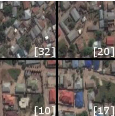
Preparatory work

Parallel to learning to understand literature, a

slightly easier task was to understand the

preparatory work done by Max in the graduation

project before this one. Reading his report and

diving into his code allowed for a better look into the

process of Max. His steps were considered in the

earliest phases of this project. His main

contributions to this project are a simple method for

creating synthetic images (examples in Figure 1

Synthetic data version 1 (Max) example) using the

Pillow fork (v6) of the PIL library for Python10_{, the}

labelled validation data (example in Figure 2 (next

page), this shows labels on top that usually are put in a separate file leaving the validation

images clean without text) and some early work using published models or derivatives of

published models to try for some results in the context of this project.

4_{https://keras.io} 5_{https://www.python.org} 6_{https://www.tensorflow.org} 7_{http://nl.releases.ubuntu.com/16.04/} 8_{https://jupyter.org/} 9_{https://www.youtube.com/playlist?list=PLZbbT5o_s2xrwRnXk_yCPtnqqo4_u2YGL} 10_{https://pillow.readthedocs.io/en/stable/}

In his experiments, Max concluded that his model

was not working as it always predicted the same

value resulting in a high error. In trying to re-use his

code, lack of documentation and issues with

versioning meant his code for training a model could

only be used as inspiration. Looking at the parts of

Keras he used in trying to define a model based on

literature, it seems there might be bugs in using the

chosen Inception networks in the current version of

Keras. This meant that for the tinkering phase

another published network has been chosen.

Max’ other work has seen more use. The code for

creating synthetic data has been adapted into something featuring more options based on

experiments and the validation data has been used throughout the whole project but will be

evaluated in the evaluation chapter.

Tinkering

As part of the course for learning to work with Keras, some assignments accompanied the

mentioned Keras tutorial series. These dealt with categorising cats versus dogs in images using

a published pre-trained network called VGG16 [16]. The same model was picked for creating a

baseline result based on a comparative study of well-known published networks [18], previous

experience in working with the model during the orientation phase and its relatively

straightforward structure. This baseline model was a standard VGG16 network with an

ImageNet [15] pre-training and featured a fully connected layer of size 768 and a dropout layer

of 35%, keeping 65% of these nodes randomly during training in the last layers. These last

layers were chosen the same as in the model used for the research of Rahnemoonfar, and

Sheppard (2017). In every layer the ReLU (Rectified Linear Unit [22]) activation was used and

for training RMSprop [23] was used as an optimizer. After some reading and seeing common

practise of people in this field it seemed this choice would yield the best results normally.

Research

Parallel to tinkering, after the first encounters with the theories behind deep learning and

ConvNets, more research went into understanding the field of deep learning and the use of

ConvNets in counting problems. It proves to be a very active and young research field. The

result of this phase was an earlier version of the state-of-the-art from which chapter 2 is derived

as well as a workplan for the second half of this 20-week-long project.

The use of most of this research would be to supply knowledge and experience for the

experimenting phase. In this phase different customized models are iteratively tested to improve

upon the baseline result. This is in line with the second path defined in the preliminary

conclusion of the state-of-the-art review. This path was chosen for several reasons. Training

using ImageNet would provide the model with filters that were too complex for the relatively

simple synthetic data used in training. In the earlier layers of the model, it was important to

experiment with different sizes of filters as it might yield an approach that would better fit the

context of this project. These experiments are documented in the next chapter. These

experiments will help in answering the research question in the end.

Requirements

In Max’ report, several requirements are mentioned and based on the requests made during this

project, his requirements are applied to this project when suitable. These requirements are

mostly about the produced code, synthetic data and model.

1. A program must be written to simulate images.

a. The images made using the program should be representative of the key

features found in the real data to provide valuable training to the deep neural

network.

b. The program must be written in Python and make use of some type of image

creation/manipulation library.

c. The code must be useable for other researchers, use clear semantics and stick

to one type of coding convention.

d. The program does not require a user interface; it is assumed that the user is

familiar with Python.

e. The program must be able to create multiple images with an amount specified by

the user.

f. The program must be able to save the generated images to a specified folder on

the user’s computer

2. A deep neural network must be created that can be trained on the simulated data and

validated on real data.

a. The neural network must be able to successfully learn to count from simulated

b. The neural network must be made using some deep learning environment

c. The neural network must be able to display its predictions to the user.

d. The predictions should be ordered by error and be displayed by the best and

worst, allowing for detection of patterns in wrong predictions.

e. The neural network must allow the user to input new data and make predictions

Chapter 5 Realisation

The realisation of this project consisted of several weeks of experiments to improve the results

of the model in predicting on the real data. The training of the model, the model itself and the

synthetic data have been improved iteratively in experiments. This chapter will show all

experiments while next chapter will evaluate on the experiments and the choices for improving

along the way. As reasoning for why experiments are done was a key aspect of this phase in

the project, reasoning of certain parts of design will be shown in this chapter, while the

evaluation in next chapter will show a discussion of results and critical notes for the experiments

in cases where things could have gone better or other choices (should) have been considered.

For the overview of all experiments see ‘Appendix 1 - model and training experiments tree’ and ‘Appendix 2 - data experiments tree’. In the first category, improvements on the model and the

training method are put. This process has been the focus in this project. Parallel to that the

synthetic data has been improved, which is documented using different versions of the synthetic

data. The experiments will be documented in chronological order. Before experiments start

using a different version of data in training, the improvements to the synthetic data will be

documented as well. Results of the experiments are evaluated using a quantifier for the error

called mean squared error (MSE), this calculation is described by the formula 𝑚𝑠𝑒 =

1

𝑛∑ (𝑌𝑖− 𝑌̂𝑖) 2 𝑛

𝑖=1 , with 𝑛 the sample size, and 𝑌𝑖− 𝑌̂𝑖 the error between label and prediction.

For this and the next chapter, training and validation graphs are put in ‘Appendix 5 – result graphs of training and validation on real data per model’. These are used as indication for the model’s performance in both training and testing (validation on real images). Training results are indicative of the model’s capability of understanding its training dataset, while testing results show the model’s capability in generalizing this training to real situations.

Baseline model

Before April – Pre-Baseline model

Using the synthetic data and validation data provided by Max and the model described in the

Tinkering section (see Appendix 3

-

a baseline performance was set. The results for this model were positive because it was able to

count the rectangles in the synthetic data accurately. In contrast, trying to generalize this

knowledge to the real data resulted in a very large error. The model failed in understanding the

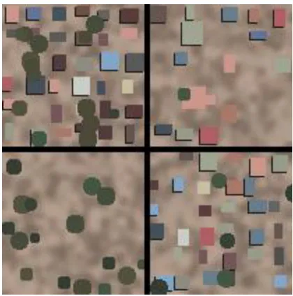
April – Synthetic data version 2, creating a more representative synthetic dataset

The goal of synthetic data is to be a feature-wise

representation of the real data. As a first step in

improving upon the results of the baseline model,

an attempt was taken at improving the synthetic

data (see examples in Figure 3) as Max’ version

was very basic. Various things were added and

improved:

• The number of generated images was

increased from 1000 to 2000. Increasing

this amount means the model sees more

diverse range of possible scenarios and

should be better at generalizing to

situations not previously encountered.

• The grid in which the houses are placed, was changed from a 5x5 grid to a 6x6 grid,

changing the image dimensions to 102x102px. Looking at the validation data, the range

in which the images are picked is between 0 and 40 houses. To create a more

representative training set, also higher density images are added to the training set.

While dealing with a regression problem should enable the model to extrapolate its

knowledge, it seemed useful to also train on high density images.

• Overlapping in generation of houses was fixed as this had been mentioned to be

undesirable in the report of Max but was still appearing in his data generation.

• The colour scheme of the data was updated to reflect the colours of the real data better,

also creating more colourful images overall.

• Using these newly picked colours, the background generation was updated to be more

representable of the background in the real data. Backgrounds are generated using the

method mentioned in Rahnemoonfar, and Sheppard (2017).

• A possibility was added to generate bigger houses. In the real data most houses are not

only rectangular, but have different shapes consisting of multiple rotated rectangles

connected to each other. These bigger houses occupy a 2x2 section of the grid and are

generated using several random rectangles in the same colour.

• Trees are randomly added to the images using colours from the real data set. This is

because trees might also be recognised as houses by the model and in this way the

training should prepare the model to distinguish between houses and trees.

• After analysing images of Tanzanian suburbs, shadows are recognized as a key feature

of the dataset. Therefore, shadows are added to the generated houses with a chance of

about 80%.

April – Baseline model

The baseline model was trained on the second version of synthetic data to create the official

baseline result. The performance of this model was used in comparison to later results to

evaluate performances of later models.

Custom model

Late April – CustomV1, defining a first custom version of the baseline

Custom model version 1 is the first custom adaptation of VGG16 (see full model architecture

template (version 2) in Appendix 4 - custom template model visualisation). Featuring two

convolutional layers of respectively 7x7 and 5x5 filter size, and a 3x3 (stride 2) max pooling

layer as first three layers. These layers were chosen inspired by the paper of Rahnemoonfar,

and Sheppard (2017). The first big convolutional layer should recognize the obvious rectangular

features of a house, while the following layers condense this information into a prediction of the

total amount of houses. Version 1 features two fully connected layers of size 768 before the last

layer, in combination with a dropout of 35% that is standard for every model from now on except

otherwise mentioned. All custom models use ReLU as activation in all layers and Adam as

optimizer for training, except otherwise mentioned.

Late April – CustomV2, testing one fully connected layer versus two

This alternative to version 1 features only one last fully connected layer with 768 nodes.

Training this model did not yield significantly different result than the first version. As the first

model contained more variables, its training used more time. Models from now on use one fully

connected layer of size 768 at the end, except otherwise mentioned.

Late April – CustomV3, testing RMSprop and sigmoid versus Adam and ReLU

This experiment tests using RMSprop [23] as optimizer and the sigmoid11 _{activation function in}

order to check their performance against the chosen Adam [24] and ReLU combination. It

shows no learning during training and after being unable to fix this problem, following

experiments use the latter, working combination.

Start of May – CustomV4, finalizing workflow and adding data augmentation

After re-evaluating the structure of the last layers, version 4 fixes an applied, but uncommon

practice. In previous versions, the output volume of the last pooling layer is directly connected to

the fully connected layers and just flattened before the dropout layer. This is changed to the

common practice of first flattening the output volume of the last pooling layer before fully

connecting these nodes. This change is also included in the baseline model before the final

baseline result is generated.

Version 4 also introduces the practice of augmenting training data. This means the model will

not only be trained on the images provided in the synthetic dataset in the way they are

generated, but also in ways that are slightly different. Augmentations that are applied (in small

amounts) are colour shifting, introducing image skewing, rotation and horizontal and vertical

flipping. This makes the generated dataset even more representative of the real world as it

should also enable the model to learn to recognise houses from the real dataset that are slightly

dissimilar to the synthetic data, for example houses that are rotated. The data augmentation is

applied in all following experiments and in the training associated to the results of the baseline

model.

May – CustomV5, testing 65% dropout rate

Version 5 is version 4 with a very high dropout rate of 65%.

May – CustomV6, replacing big convolutional layers with several smaller convolutional

layers

Version 6 tries to implement a practice to decrease the number of variables in a network by

replacing the big convolutional layers with smaller ones. The two first, large convolutional layers

are replaced by 3 3x3 convolutional layers. This is not exactly equivalent as 3 3x3 layers

resemble only one 7x7, but this simplification is also part of the experiment.

May – CustomV7, testing version 4 with two convolutional layers

Version 7 is version 4 with two fully connected layers, like version 1.

May – CustomV8, testing 65% dropout rate under new training variables

Version 8 is the same as version 5, but before training, the training variables are tuned and

learning rate is decreased. For the first time predictions are visualised to see what the model

May – CustomV9, comparing 50% dropout rate to 65%

Version 9 is version 8 with a dropout of 50%. The prediction visualisation is expanded by a

visualisation of the best and worst predictions for the validation data. From now on, this is used

to find common features in the worst predictions to improve the training process and synthetic

data.

Late May – CustomV10, comparing 35% dropout rate to 50% and 65%

Version 10 is version 4 under training conditions of version 8. Five iterations of improving the

synthetic data are done using this experimental setup.

Late May – Synthetic data version 3, testing small improvements to version 2 data

Several additions and improvements are implemented in the code for generating synthetic data,

testing the effect by training the custom model 10 and reviewing the results of predicting on the

validation dataset.

Version 3.1, introducing larger (n=10k) set and adding grass to background

• Implements randomized grass coloured shapes in the background

• Puts trees on grid between houses to prevent putting trees in houses, trees are still

allowed to overlap houses and can appear in big houses as they occupy a 2x2

section of the grid

Version 3.2, large set improves generation of grass, trees and small houses

• Improves grass creation by randomizing generated shapes better

• Increases smallest size of small houses

• Implements switch statement for generating images with relatively few trees versus

images with relatively large amount of trees

Version 3.3, small set to test adding more green colour to background

• Implements switch statement for the colours used in background and grass creation,

resulting in sand-coloured backgrounds with grass patches (standard) and green

backgrounds with sand patches

• Improves big house generation by assuring that big house segments are always

Version 3.4, small set to test blurring final image

• Puts a final blur over the generated image

Version 3.5, large set without blur to test adding fences to data

• Removes blur from version 3.4

• Implements random shadow coloured lines in the image to resemble fences

June – CustomV11, test stride (5, 5) in the first convolutional layer

Version 11 is the first in a row of experiments that change the stride value in the first few layers.

This version implements a stride (5, 5) for the first 7x7 convolutional layer. A bigger stride would

allow the model to scan the images with less overlapping filters and this could help in situations

where the model counts houses twice. Implementing a stride makes the output of a layer

smaller as less output values are generated. In this experiment the structure of the model is not

changed other than its first layer.

June – CustomV12, test stride (3, 3) in two first layers

Version 12 implements strides of (3, 3) in both first convolutional layers. As this decreases the

output volume significantly, the first max pooling layer is removed, and the final fully connected

layer is decreased in size to 256 nodes.

June – CustomV13, test stride (4, 4) in two first layers

This experiment tests the impact of stride (4, 4) in the first layer of version 12.

June – CustomV14, stride (5, 5) in two first layers with shallower model

This experiment tests the impact of stride (5, 5) in the first layer of version 12. It removes a set

of 2 3x3 convolutional layers and a 2x2 max pooling layer at the end to account for a decrease

in output volume of the earlier layers.

End of June – Synthetic data version 3.6, test removing additional green in the

background

Combining the best results of the experiments with custom model version 10, a synthetic data

version was created in which the switch for green with sand patches background was removed

End of June – CustomV12 with linear regression model

Together with using the data version 3.6 in combination with custom model version 12, which

produces the best results yet. This model combines the deep convolutional neural network with

a linear regression model. Taking the output of the ConvNet and putting it through a linear

regression model yields the final prediction. The linear regression model is implemented using

the LinearRegression class from the scikit-learn (v.0.21.2) library12_.

Chapter 6 Evaluation

The first part of this chapter follows up on chapter 5, where all experiments and their structural

changes were described. This will explain design choices, mention decisions considering the

flow of the project, discuss errors made in the experiments and finally evaluates the project.

Per model

Per model the thoughts behind the experiments and some reconsiderations after the fact are

described.

Pre-Baseline model

The pre-baseline model acts as the first baseline. However, as the workflow for saving results is

not yet defined during this experiment, recordings of this experiment are made afterwards. After

this first result experimental iterations are already made, defeating the purpose of a baseline in

one way, but providing a more representative result as a baseline in the end.

It is concluded after seeing the performance of this model that it has a very hard time

interpreting the real data. And thus, a more detailed and complex version of synthetic data is

tested.

Synthetic data version 2

In the second version of the synthetic data several drastic changes are made to the synthetic

data. These have not all been individually tested. When tested they were not recorded for the

same reason of the pre-baseline model. The changes made to the data are ones that do not

always follow from findings in experiments, but rather follow from intuition about learning in deep

learning models and trying to make the synthetic data more representable of the real data

based on what is seen in this real data.

Baseline model

The baseline model knows several iterations before becoming a baseline result. This is the

result of being thrown in the deep quite quickly after a relatively short tinkering phase. In this

tinkering phase, practices around training a ConvNet were still very new and several base

requirements had to be met before continuing to the experiments phase. While setting up the

training environment properly and implementing ways to save the results of the experiments,

some attention also went out to improving the synthetic data. As the workflow that allowed

further experiments to take place was refined enough, the synthetic data had been improved

baseline result of generalisation to real data very much by decreasing the error in case of

testing the model on real data.

CustomV1

This model was defined because training from scratch without the pre-training on the ImageNet

data was preferred but difficult with the via Keras implemented VGG16 network. The

pre-training of the model based on the ImageNet data equipped the model with very good filters for

looking at data that is found in the ImageNet database. The ImageNet dataset mostly consists

of real images of organic objects, like cats and dogs, or real-life objects, like cars and boats. In

the tinkering phase with the categorization problem of cats and dogs, this allowed the model to

quickly apply its pre-training to the supplied organic retraining data and allowed for achieving a

high accuracy. However, the synthetic data in this project requires another sort of filters as it is

mostly made up of simple colours and simple shapes. Using the advanced pre-trained

knowledge would probably introduce too much knowledge of the real world and disallow the

model to distinguish only houses.

CustomV2

As different models in literature used multiple fully connected layers in the end to arrive at a

conclusion, the first model was compared to the second to see if this would also improve the

results in this case. Using less variables did not influence the results significantly and caused

shorter training times. This led to the conclusion of making this the standard.

CustomV3

The third experiment would have been very useful if executed correctly. The reason this version

would not converge during training was that the input images were not normalized. This

normalization will only find place after trying to use sigmoid on version 12 and understanding

that sigmoid cannot deal with the values in the network in the same way as ReLU can. Sigmoid

deals with numbers between 0 and 1 and ReLU functions between 0 and the maximum number

at that moment. This means, the experiments are still valid, but this experiment has no value as

it fails to compare two setups. It shows however, that applying sigmoid to a regression model

might be complicated as outputs of predictions are not between 0 and 1 and therefore the model

is unable to decrease its error.

CustomV4

In the fourth experiment the final layers are implemented properly. Due to this error the earlier

models should only be taken as indication. Additionally, to enhance training, the synthetic

example. The introduction of this data augmentation means the data is very diverse and thus

creates a more challenging training environment. This results in a high error in validating on real

images.

CustomV5

This experiment tries to make generalization better by using a very large dropout value. This

65% was suggested by the supervisor because of its mention in the paper of Rahnemoonfar,

and Sheppard (2017). However, what they meant with the dropout value of 65% they use (which

they mention under section 4.1), is what they explain at the end of section 3.4 where they

mention that “[s]ixty-five percent of connections were randomly kept while training the network.”

As version 4 and 5 both show similar results and training on the synthetic data seems even

more difficult for this model, this experiment fails to show the usefulness of such high dropout

value.

CustomV6

In networks like Inception and VGG only convolutional layers with small filters of 3x3 are used to

represent larger filters, stacking two 3x3 convolutional layers should perform similar to a 5x5

convolutional layer, but saves on quite a bit of variables [16, section 2.3]. This experiment tests

this by replacing the first two convolutional layers by 3 3x3 convolutional layers. This is not a

one-to-one conversion, but also tests if maybe a shallower option would perform better. Training

this model is easier, but its results are slightly worse than the models with the large

convolutional layers.

CustomV7

Like the first experiment, this one tests if more fully connected layers at the end could improve

the results. Here it seems to matter as in comparison to version 4, the training converges better

and the result has a smaller error. Although version 7 improves upon version 4, implementing a

second fully connected layer did not prove useful for the final version 12.

CustomV8

The error in all previous custom experiments has never been smaller than the baseline result in

experiments with a model that would be comparable and adheres to common practice around

fully connected layers. Therefore version 8 tries to improve the result of version 5 by decreasing

the learning rate in training (to 0.0001) to see if this means the model will be more successful in

training valuable knowledge. From the results it seems the model is now performing much better

are defined to see the result of smaller dropout values, as this one still uses the extreme

dropout value that was not proven useful in version 5.

CustomV9

Using the new training setup from version 8, this experiment tries version 4 with a dropout of

50%. This is the most extreme dropout value tested in Rahnemoonfar, and Sheppard (2017),

which was not picked as it showed worse performance than the value of 35%. To improve the

results of this and future experiments, a best versus worst visualisation is added. In analysing

the worst images for common features, representing these features in the synthetic data might

prepare the model better for future predictions. This is what happens in the next experiment.

CustomV10

This experiment is the exact same as version 4 but uses the improved training variables

introduced in version 8. The dropout value of 35% means training is not too challenging to

perform well on real data. The performance of this model trained on the second version of the

synthetic data is an improvement over the baseline result. To see if this can be improved

further, the synthetic data is modified five times to improve the predictions on the real data.

Synthetic data version 3

Because testing the model has led to a model that performs better than the baseline model,

several tests are run with a new version of synthetic data. These experiments aim to improve

the models feature recognition in the real data, to prevent false positives and counting features

that are not houses.

Version 3.1

In the background of the real images, this new version adds some randomized green

patches in the background to prepare the model for houses that might be placed on

grass and could stay undetected before. Putting the trees on the grid cleans up the

training set by preventing houses to be overlapped too much by the random placement

of the trees which would make it more difficult for the model to know what it is exactly

counting. The new method allows only partial overlapping of small houses as the trees

will only be put between houses, overlapping only with some of their foliage.

Version 3.2

To improve the training set more, the changes in the May version 1 data are tuned

slightly. A different tree generation method is tested to allow for a better representation

on images of regular suburban areas with about 15 – 25 houses on them. Worst

predictions after training on both first versions of data are unclear images with high

density areas (30+ houses), images of green areas with less than 5 houses and images

that feature a road or fenced areas. Both first sets are 10k images large and this allows

for better training.

Version 3.3

Implementing a switch between green with sand patches background and the standard

sand with green patches background is tested. The reason for this change is that there

are several images with no houses on them in the validation set, that have high counts

as predictions. However, after training on this set, the results do not show this

improvement convincingly.

Version 3.4

To imitate the blur apparent on most images in the validation set, this experimental

dataset tests the effect of blurring the synthetic data. The results are worse than the

other version 3 datasets, but the model performs well on the high-density images that

are the most unclear images of the dataset. This shows that it might be possible to deal

with images of lower resolutions by creating low resolution training data.

Version 3.5

To achieve better results the final test on version 10 adds fences to the May version 3

images. This improves the results of the model slightly and proves that adding features

to the data can be useful to prepare the model for these features in the real dataset.

However, the overall improvement achieved by this tinkering with the data is smaller

than initially hoped and the model is not yet capable enough to give good indications of

the number of houses found on the images in the dataset.

CustomV11

Trying to improve the predictions of the model, a new set of experiments is defined. In these last

experiments the first layers are tested with different strides. A different stride could help to scan

for only houses better and would prevent double counting if that would occur, although double

counting did probably not occur in most cases as it was not found in analysing the worst results.

This version has similar results to version 10 trained on blurred synthetic data version 3 (May

version 4).

Applying a less extreme stride to the first two convolutional layers is tested against version 11

and shows much better results. Analysing the worst predictions introduces the suspicion that the

validation data is labelled incorrectly in some cases and some of the predictions make more

sense than the labelling itself. A new labelling is made, but as there is no documentation on

what should be labelled, this labelling is too strict and does not improve the results.

Version 12 is also tested with sigmoid activations and upon better inspection shows the need for

normalisation of the input data as mentioned in version 3. No new sigmoid experiments are

carried out after applying the normalisation.

CustomV13 and CustomV14

Both version 13 and 14 make use of the new, strict labelling. Comparing to version 12, these

experiments both predict better on this interpretation of the validation dataset. To test against

version 12, bigger strides are applied for the first layer. For version 14 the results are interesting

as its structure has been modified quite heavily, making the model shallower than the others.

The findings of these experiments are not comparable to the rest of the experiments as they use

a different validation labelling.

Synthetic data version 3.6

Evaluating the results of tests with the five earlier mentioned version 3 datasets, dataset 6 is

defined. Using a 10k large dataset is required in training the latter models and a bigger set could

be even better, although not tested. The change from May version 3 with the switch for

background colours is removed as this introduced an error and removing it should lead to the

best results yet.

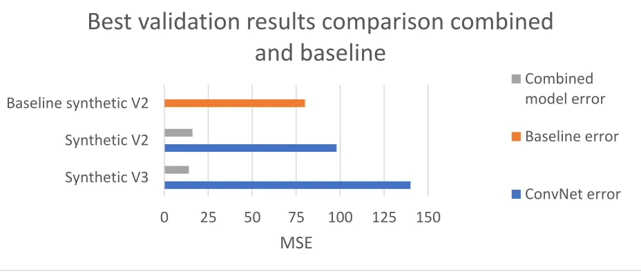
CustomV12 with linear regression model

Analysing the final predictions, a certain trend is recognized. This probably means that the

model can roughly estimate the number of houses but also encounters uncommon features in

the validation data that influence the final prediction. This trend could be resolved applying a

linear regression model after the deep learning model. Applying this linear model, yields the

best results yet. As the final solution, this combination of models achieves a validation error of

average. The results for this model are shown in Figure 4 (next page). This model provides a

satisfactory indication of the amount to houses in real-world images based on synthetic training.

Figure 4 Best validation results combined model (for v2 versus v3 synthetic data)

0

25

50

75

100

125

150

Synthetic V3

Synthetic V2

Baseline synthetic V2

MSE

Best validation results comparison combined

and baseline

Combined

model error

Baseline error

Project

The project is evaluated in three different parts: preparation, experimentation and evaluation.

Preparation

At the start of this project, a lot of preparatory work had to be done. The work of Max was

supplied, but there was no documentation on his code, which limited the ability of transferring

his work. Due to a lack of experience and knowledge in this field, the initial research was very

broad and forming an intuition was a tough task. After several guided tutorials and reading

about the matter, a basic knowledge and skill was acquired which served as the preparation and

introduction to the subject matter.

Experimentation

Experiments at the start of this phase are more tinkering than guided experiments and find

place under conditions that allow the results to only be indicative. The earlier experiments

provide an environment that enables the following experiments to take place and produce

results. Throughout the project errors are made due to inexperience and lack of knowledge. At

the end of the project, training some of the earlier recorded models again, the results differ from

the ones recorded when doing the experiments for the first time. However, a certain intuition

and skill in doing experiments with ConvNets is acquired and finally a good result is achieved.

Evaluation

Due to the complexity of the problem, the experiments took place till right before the final

presentation and sometimes left little room to evaluate properly in between. This should

sometimes have gotten more attention, which would have allowed for a more focused and

organised approach. Evaluating at the end, the process to a solution is also a process of

learning to understand just a bit about deep learning with ConvNets. This is not a bad thing but

Chapter 7 – Conclusion

In the conclusion, an answer to the main research question should be defined based on the

findings of the project. The research question will be repeated here for clarity:

In what way should a deep convolutional neural network be designed to train on synthetic data

in a regression problem dealing with counting while being able to generalize its knowledge well

in real-world test situations?

First, it should be mentioned that this project only provides start of an answer to this question

and that research in this area is evolving in the meantime to propose new and innovative ways

which define better answers to this question already. Some of these will be mentioned in the

next chapter.

This research compares transfer-learning a published model, VGG16, to a custom-built model

that implements and tests some suggestions from other research done in this area. From this

comparation, it is concluded that creating a customized model, while complicated, probably

yields a better solution to a specific problem than a general published network.

Key findings in this research project are about synthetic data (1) and creating a custom model

(2).

1. Starting with a very simple synthetic dataset (version 1) to train a deep ConvNet to train

it for looking at complicated real data is not very effective. Training on more

representative and more complex synthetic data provides a better result when testing

the model on real data. Designing synthetic data is a complicated task and should be

done while iteratively testing the alterations made to the data. Keeping in mind that

adding features in the synthetic data also creates a more challenging training

environment.

2. One of the biggest challenges in creating a custom model is overfitting. Applying a

dropout and some structural decisions about small fully connected layers help in battling

this. Using big filters and strides in the earlier layers in the final model seem beneficial to

the model’s capability in predicting on real data. Training variables, like learning rate, are

an important part of the model optimisation.

In the end a model is defined that can indicate the number of houses on images in the provided

validation dataset. After the output of the deep learning model, a linear regression model is

of 3 on average. This performance is acceptable for the purposes of this project in this

experimental setting and with the provided validation set.

The requirements mentioned in Requirements are met by designing a custom model capable of

indicating the amount of houses on real data images, based on training with generated synthetic

data representative of this type of real data. Additionally, the code produced in this project will

be made retrievable and will be clean and documented well enough for learned users to be able

Chapter 8 – Future Work

While this work presents a final experimental, customised model that performs acceptably,

better results can be achieved by taking this work further and experimenting within this context

in a more structured way and with better contextual data. Several recommendations for future

work are defined:

1. Before building on this research, define a better, higher resolution validation dataset. As

this dataset is key part of this research, significantly more attention should be given to

acquiring and labelling this data, before continuing to experiment with models to test on

this data. The current validation dataset should not be reused without an effort to better

define and document the ground truth for this context.

2. In this project a very simple way of generating synthetic data is chosen to investigate.

Using this basic generation, improvements are made resulting in a synthetic dataset that

is more representative of the real data, but still quite abstract. This might limit the

model’s capability to understand the real data and might not be the best approach in this

sort of problems that deal with more complicated or diverse real data. Other methods

also considerable for future work: a hybrid version using cut out houses from real

situations, similar to the validation data or generating data using 3D programs [25] or

more realistic generation tools than the one used in this project.

3. Counting problems are quite new problems and the applied method of training the model

to count is just one of the possibilities. Another quite new and promising method of

counting uses training to generate density maps from input images, of which predictions

for the count are made instead of directly inferring the count from the image [26]. This

could be investigated in a context like the one in this project, by counting houses on

satellite images of bigger parts of cities instead of in the range of 40 houses.

4. The method of stacking two different models to arrive at better predictions should be

kept in mind when continuing this work. Using clearer validation images might already

solve the need for this practice, but in this project it allowed for a much better result in

the end.

After this project the accompanying code and datasets are made accessible for future work.

Mail the author of this report or the supervisor if there is interest in the code, datasets or other

Appendix 1 - model and training experiments tree

Baseline model VGG16, ImageNet pre-training,

FC768, DO35 Use Adam optimizer, ReLu activation from for following

experiments

CustomV1, simplified own version of VGG16, 2x FC768,

DO35

CustomV2, like V1 but 1x FC768

CustomV4, like V2 but uses proper flattening before last FC

layer.

Use data augmentation from now on

CustomV5 test V4 with DO65 CustomV7, test V4 with 2 FC layers

CustomV8 test V4 with DO65 but (from now on) better training variables (learning rate)

CustomV9 test V4 with DO50 and slightly tuned image input

size

CustomV10 test V4 with DO35

Trained using 5 improving versions of synthetic data

CustomV3, test V2 with RMSProp optimizer and sigmoid

activation

CustomV6, replace starting 7x7 and 5x5 by 3 3x3 convolutional

layers

CustomV11, V4 with stride 5 in first convolutional layer

CustomV12, improves on V11, stride 3 in first and second convolutional layer, FC256 instead of FC768, removes first

3x3 stride 2 max pooling layer

CustomV12 with added Linear Regression model CustomV13, V12 with stride 4 in

first layer