warwick.ac.uk/lib-publications
A Thesis Submitted for the Degree of PhD at the University of Warwick
Permanent WRAP URL:
http://wrap.warwick.ac.uk/78992
Copyright and reuse:
This thesis is made available online and is protected by original copyright.
Please scroll down to view the document itself.
Please refer to the repository record for this item for information to help you to cite it.
Our policy information is available from the repository home page.
M A E
G
NS I
T A T MOLEM
U N
IV ER
SITAS WARWICEN
SIS
Primitive stability and Bowditch conditions for
rank 2 free group representations
by
Damiano Lupi
Thesis
Submitted to the University of Warwick
for the degree of
Doctor of Philosophy
Department of Mathematics
Contents
Acknowledgments iii
Declarations v
Abstract vi
Chapter 1 Introduction 1
Chapter 2 BQ and PS 5
2.1 Free groups and primitive words . . . 5
2.2 Character variety . . . 7
2.3 Bowditch conditions . . . 7
2.4 Primitive stability . . . 8
2.4.1 The mapτρ,O . . . 8
2.4.2 Bi-infinite geodesics and uniformity . . . 8
2.5 Sufficient conditions for primitive stability . . . 10
2.5.1 PS ⇒ BQ . . . 10
2.5.2 Two more conditions . . . 12
Chapter 3 Primitive stability and tessellations of the hyperbolic plane 15 Chapter 4 Real representations, BQ conditions and primitive stabil-ity 24 4.1 Three real traces imply Fuchsian . . . 24
4.2 The action ofOut(F2) . . . 25
4.3 Ergodicity and BQ conditions . . . 30
Chapter 5 The diagonal slice ∆ 33 5.1 The slice and its symmetries . . . 33
Chapter 6 Pleating rays and boundaries of PS ∩∆ 38
6.1 A bit of pleating ray theory . . . 38 6.2 Rational case: lifted curves are blocking . . . 42
Acknowledgments
The present work is the result of an experience which started four years ago, and
that has seen many people contributing to my scientific research and personal
de-velopment.
A first, enormous thank goes to my supervisor, Prof. Caroline Series, who
guided me through this compelling adventure, from when I was moving my first
steps in the hyperbolic world until the very last reviews of the thesis. Thanks to
her, I could learn about this fascinating subject, discover the thoughts of the greatest
minds in the field, and find the little researcher hidden in my personality.
I want to thank my examiners, Brian Bowditch and Jack Button, for reading
my thesis and showing interest in my research.
Research ideas come from sharing thoughts and communicating with others:
for this reason, I am deeply grateful to the geometry and topology team of the
Uni-versity of Warwick, namely Caroline Series, Brian Bowditch, Saul Schleimer, Karen
Vogtmann, and their Ph.D. and post-doctoral students, with whom I had long,
pleasant hours of conversation, and who taught me how to think like a topologist.
I would like to thank all the people who keep believing in the power of human
imagination and creativity.
Finally, I would like to express my sincere, deepest gratitude to my family
and friends. They never gave up supporting and encouraging me. They shared my
Declarations
This thesis is submitted to the University of Warwick in support of my application
for the degree of Doctor of Philosophy. It has been composed by myself and has
not been submitted in any previous application for any degree. The work presented
(including data generated and data analysis) was carried out by the author, except
in the case of Figure 5.1, which has been originally produced by C. Series, S. P. Tan
Abstract
We introduce two different properties of representations of the free group of rank
2 into the group of hyperbolic isometriesPSL(2,C): BQ conditions and primitive
stability. We investigate relations between the sets of characters satisfying these
conditions, and study certain slices of the character variety separately. The results
we get are in line with the conjecture that these two sets actually coincide. We
also show that in the diagonal slice of the character variety, namely the set of
representations with associated trace triple (z, z, z), z∈C, there exists a large class
Chapter 1
Introduction
Hyperbolic manifolds have been a big source of interest and study in the last decades. The idea of a hyperbolic geometry was born in the first half of the nineteenth century.
From the very first definitions in the context of complex analysis, this rich branch of
mathematics gradually developed mainly in three directions, trying to understand and explain various phenomena that can be partitioned into three big classes: the
theory of complex variables and conformal mappings, the topology of hyperbolic
manifolds and the combinatorics of groups. The three brilliant minds contributing to these different yet intertwined fields belong to Henri Poincar´e, and his original ideas
from where most of the theory originated, William Thurston, with his remarkable
geometrisation conjecture, and Mikhail Gromov, with his coarse point of view on geometric group theory.
In this thesis, we shall mainly focus on the topology of hyperbolic surfaces
and 3-manifolds and, to a smaller extent, on some group theoretical features of the free groups. A hyperbolic orbifold can be described as the quotient of the hyperbolic
space under the action of a discrete group of isometries. Such a group is called a
Kleinian group. If the group is also torsion-free, then the quotient is a hyperbolic manifold. For this reason, the geometry of hyperbolic orbifolds and the algebra of
Kleinian groups are deeply related.
Hyperbolic isometries are bijectively associated to elements in the group
PSL(2,C), and therefore they can be thought of as (classes of) matrices. When
we want to analyse many isomorphic Kleinian groups (isomorphic in the classical
sense, that is in the category of groups), a very powerful tool is to think of them as images of the abstract group to which they are isomorphic. That is, we fix
a group and consider its representations into PSL(2,C). In other words, we are
an “external” group. This is the most natural setting to allow deformations of Kleinian groups. Deforming a Kleinian group roughly means continuously varying the image of a fixed abstract group into the space of hyperbolic isometries. Now
that a Kleinian group has been replaced by amap, the next natural step to take is to consider the space of all of these maps. For an abstract groupG, we form the space Hom(G,PSL(2,C))//PSL(2,C) of (roughly) conjugacy classes of homomorphisms
fromGto the group of hyperbolic isometries, and call itcharacter variety. We shall be interested in the very special case whereG is a free group of rank 2.
We shall be interested in subsets of the character variety satisfying certain
specific conditions.
The first subset we shall encounter is that of the representations satisfying BQ conditions, or Bowditch conditions (see Definition 2.4 for a definition). We
shall denote this open subset by the symbol BQ. BQ conditions were introduced
by Bowditch in [Bow]. In this paper, the author analyses connections between
Markoff triples and representations of the free group of rank 2, and proves that in
the subset of characters satisfying BQ conditions, some identity “`a la McShane”
holds. The same subspace is deeply studied in [TWZ], where the authors obtain a further extension of McShane’s identity and prove that the mapping class group
of the torus acts properly discontinuously on it. BQ conditions can be described purely in terms of traces of matrices, and can be therefore considered algebraic in
flavour. Nevertheless, the trace of a loxodromic element matrix has an important
interpretation in terms of its translation length, and we shall see the geometrical repercussions of this key fact.
On the geometrical side of the game, instead, lies a different property of
characters, called primitive stability. This concept was introduced by Minsky in [Min] and it is basically has to do with hyperbolic geometry, being defined in
terms of Cayley graphs, metrics and quasi geodesics (see Definition 2.7). In [Min],
the author is interested in studying the dynamics of the action of Out(Fn), the
outer automorphism group of the free group of rank n, on the character variety
Hom(Fn,PSL(2,C))//PSL(2,C). The main theorem of the paper states the
ex-istence of an open subset of the character variety, strictly larger than the set of Schottky representations, whereOut(Fn) acts properly discontinuously. This is
ex-actly the subset of primitive stable characters, that we shall denote byPS.
Rather oddly (or maybe not!) when n = 2, Out(F2) is isomorphic to the
mapping class group of the torus. Moreover, both BQ and PS are open sets and
contain all the Schottky characters. Assuming that there may be a correlation
main conjectures in this topic, that is PS = BQ. This conjecture doesn’t seem to
be proved so far. Another important open conjecture, made by Bowditch, states that, in the case of representations of F2 where the commutator element is sent to
a parabolic, BQ conditions correspond to quasi Fuchsian representations. Although
both conjectures seem to be still open at the time of writing, we shall give an ar-gument to see that primitive stability implies BQ conditions, and shall prove that
PS also contains a class of representations which is larger than Schottky
charac-ters, reinforcing Minsky’s observation. These preliminary results will be exposed in Chapter 2.
As often occurs in mathematics, when one has to tackle a problem in a space
that is too big and complicated to be analysed at once, a clever way of proceeding is to restrict to a few subcases and try to solve the problem within these easier settings
first, hoping that they might be correlated and eventually they could reveal the big
picture. Investigating BQ conditions and primitive stability in the whole character variety is a hard task. In order to work in a smaller, more easily understandable
setting, we will play this trick and focus our efforts on some specific subsets.
In Chapter 3, we only consider representations whose image is contained in
PSL(2,R). This allows us to work with two dimensional hyperbolic geometry, and
to develop some technique to prove primitive stability only by looking at the trace of the commutator element.
Ifaandbform a pair of generators of the free group of rank 2, the conjugacy
class of a character is uniquely determined by the three complex values of the traces of the image matrices corresponding to a, b and ab. This allows us to identify the
character variety with the complex vector space C3. The identification with C3
helps us in easily slicing the variety again. If the triple of traces is real, for instance, we say that the associated character is areal representation. Thus, the subspace of real representations can be seen as the real three-dimensional vector space sitting
inside the complex one, R3 ⊆ C3. We shall analyse primitive stability and BQ
conditions in this space in Chapter 4, following the outline that Goldman gives in
[Gol2], and using many of his results. In [Gol2], the author carefully analyses real
representations by looking at the trace of the commutator element, and studies how the action of the mapping class group changes according to this trace. Combining
his deep analysis with our result from Chapter 2, we describe a precise way to know
whether or not a representation is primitive stable.
The other subspace we shall analyse is the diagonal slice. This slice corre-sponds to characters identified by triples of traces with the same complex value. If
geom-etry, here what helps us is symmetry: the peculiar configuration of the traces tells
us that, in the Kleinian case at least, the quotient manifold is a genus 2 handlebody with a special rotational three-fold symmetry. Moreover, since any triple in the
diagonal slice can be specified by giving just one complex parameter, it can also be
plotted and visualised easily.
Firstly, in Chapter 5, after introducing the slice and explaining its
symme-tries, we apply our previous results about real representations to the real line and
get a first overview.
In Chapter 6, finally, we deal with the rest of the slice. In [Min], the author
shows that Schottky characters are primitive stable, and also that primitive stable
representations form a strictly bigger set than Schottky characters. These last ones form an open set in the character variety, and are also the interior of the closed set
of discrete and free representations. Our main result shows that there exists a rather
large set of primitive stable representations which are not discrete nor free. The very special situation of the diagonal slice gives us a way of easily classifying the curves on
the boundary of the handlebody which are invariant under the rotational symmetry.
By using the machinery of pleating rays, we shall describe some of the points on the boundary of the discrete and free locus as endpoints of appropriate pleating
rays, which correspond to bending these symmetric curves. Recent results obtained by Jeon and Kim about geometrically infinite representations in the boundary will
Chapter 2
BQ
and
PS
The main definitions and concepts are presented here. The reader who is well
acquainted with the topic may want to skip this chapter. For completeness, we
give a proof of the fact that the set PS is contained in BQ: it is a very
straight-forward conclusion, but apparently it nowhere appears in the literature. We also state two more sufficient conditions to conclude that a representation is primitive
stable (Proposition 2.11 and Corollary 2.14), since we shall use them extensively
later on.
2.1
Free groups and primitive words
Afree group of rank 2 can be defined by the following standard presentation:
F2=ha, b|·i.
Namely, it is the group generated by two elements, say aand b, with no relations.
Probably the easiest way to think of it, as a set, is as the set of words in the alphabet a,b,AandB, where AandB denote, respectively, the inverses ofaand b. For this
reason, we will often use the term word to describe an element of the free group. The identity element is the empty word, made of no letters. The group operation is simply the juxtaposition of words. A word where no letter followed by its inverse
appears, is calledreduced. If the first letter of a reduced word differs from the inverse of the last letter, then we say that the word iscyclically reduced.
Thelength of a word, with respect to the generatorsaandb, is the number of letters that the word is formed by, after reduction. The length of the empty word is zero.
generating pair. Primitive words will be crucial for us. In a free group of rank 2,
primitive words can be written in a very special form, that will be very important later on. The typical pattern of a primitive word inF2 is described in the following
theorem.
Theorem 2.1 ([CMZ]). Suppose that some conjugate of v=an1bm1. . . anqbmq and
some conjugate ofw=aα1bβ1. . . aαpbβp form a basis of F
2, wherep, q≥1and all of
the indicated exponents are non-zero. Then, modulo trivial changes of notation (the possible replacement of a by a−1 or b by b−1, throughout), there are integers n >0
andε=±1 such that either:
m1=. . .=mq=εβ1 =. . .=εβp = 1, {n1, . . . , nq, εα1, . . . , εαp}={n, n+ 1}
or, symmetrically,
n1 =. . .=nq=εα1=. . .=εαp= 1, {m1, . . . , mq, εβ1, . . . , εβp}={n, n+ 1}.
Remark 2.2. It is worthwhile making a crucial observation here: by the theorem above, a cyclically reduced primitive word can only have a very special pattern:
• only two of the symbols from the alphabet {a, b, A, B} appear,
• one of the two always occurs as an isolated letter, i.e. with exponent either always equal to 1 or always equal to−1,
• the powers of the other letter always have exponents belonging to {K, K+ 1}, where K can be any integer number.
One could actually go further and prove that the patterns we see in primitive words in F2 actually form what is called a balanced sequence, but this goes beyond the
purposes of this thesis. The interested reader can find more details in [Ser].
Since we will need a few more definitions about words in the free group later,
it is worth giving them here: we say that a word is primitive-blocking if it never occurs as a subword of a cyclically reduced primitive word in F2. We say that a
word is blocking if one of its powers is primitive blocking.
Example 2.3. The word w(a, b) =ab2ais blocking, since its second powerab2a2b2a
Checking that an element in a free group is blocking is not always a simple
task, and one efficient technique to determine this property is to look at the asso-ciated Whitehead graph. We shall explain later on what these graphs are and how
they can help us.
2.2
Character variety
Since we shall study representations of the free group of rank 2 into the group
of isometries of the hyperbolic space, it is convenient to consider the set of all these maps. As usual, we want to distinguish between two such maps only if they
significantly differ, namely, if their images are not just conjugate. For this reason,
the natural space to consider is thecharacter variety defined as:
χ=Hom(F2,PSL(2,C))//SL(2,C),
where the quotient has to be intended in the geometrical sense, that is classes in the
quotient are closures of orbits under the action ofSL(2,C) via conjugacy.
It is well known that there exists a bijection between points inχ and triples inC3.
This correspondence is given by assigning to a representationρ∈Hom(F2,PSL(2,C))
the triple of traces (tr(ρ(a)), tr(ρ(b), tr(ρ(ab))∈C3. Since traces are invariant under
conjugation, and representations with the same associated triple must be conjugate,
this settles a bijection between points inχ(i.e. classes of representations) and points
inC3. In what follows, we will often deal with a fixed representation instead of its
class in χ; the reader will immediately realise that all the definitions and concepts
involved are invariant under conjugacy.
2.3
Bowditch conditions
Bowditch conditions (often shortened to BQ conditions) were introduced by Bowditch
in [Bow], and analysed in deeper details in [TWZ]. The definition we will make use of is the following:
Definition 2.4 (BQ conditions). We say that ρ:F2→ PSL(2,C) satisfies the BQ
conditions if
• the image of every primitive element is a loxodromic isometry and
• the inequality
holds only for a finite number of (conjugacy classes of ) elements of F2.
Remark 2.5. Observe that the two conditions above are invariant under conjugacy in PSL(2,C), hence it makes sense to speak about classes in the character variety
satisfying these requirements. The second BQ condition, in particular, implies that the absolute values of traces of primitive elements do not accumulate anywhere in
R, that is we can replace the 2 in the inequality with any positive constant. This
result has been proved by Bowditch and follows from Theorem 2 in [Bow]. This fact is highly non trivial, and the original argument makes use of the notion of Fibonacci growth for certain maps associated to Markoff triples. This machinery involves a number of topics and technicalities which go beyond the purpose of this paper. The interested reader can find more details in [Bow] and [TWZ], for instance.
Denote byBQthe subspace of the character variety where the BQ conditions
hold.
2.4
Primitive stability
2.4.1 The map τρ,O
Letρbe a homomorphism fromF2 toPSL(2,C),O a point in the hyperbolic space
H3 andC(F2) the Cayley graph ofF2 relative to a fixed pair of generators, equipped with the standard word metric (each edge has length one). We denote byτρ,O the
uniqueρ-equivariant map fromC(F2) toH3, sending the vertex w toρ(w)·O and
the edge (w1, w2) to the geodesic segment betweenρ(w1)·O and ρ(w2)·O. We will need often to label the edges of the Cayley graph, and similarly of its image under
the map τρ,O, in order to keep track of paths in the graph. If (g, h) is an edge in
C(F2), we assign to it the label g−1h. We use this peculiar labelling convention
to keep the labelling system “equivariant” under the action of the group. For, if
g = e1. . . en and h = e1. . . enen+1, where ei ∈ {a, b, A, B}, then the edge (g, h) is
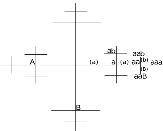
labelled by en+1. Consistently, the edge g−1 ·(g, h) = (11, en+1) is also labelled by en+1. Figure 2.1 shows the labelling convention for a portion of the Cayley graph.
2.4.2 Bi-infinite geodesics and uniformity
Consider a cyclically reduced primitive elementw∈F2and associate to its conjugacy class a bi-infinite word ¯w =. . . www . . .. If we think about F2 as the fundamental
group of a wedge of two oriented circles with labelsaandb, it is easy to see that ¯w
a
b
A
B
a
aa
a
abaaa
a
aB
(a)
(B)
[image:17.595.190.459.120.336.2](a) (b)
Figure 2.1: Edge labels are in brackets.
path to the universal cover of the wedge, namely the Cayley graph of F2. ηw is a
family of arcs inC(F2), and its image viaτρ,O is a family of broken geodesics in the
hyperbolic space, that we denote byGw.
Definition 2.6 (Quasi geodesics). Let γ =. . . , vj−1, vj, vj+1, . . . be a curve in the
Cayley graph of F2, that is an infinite sequence of adjacent vertices in the graph
(note that, to avoid repetitions in the sequence, we do not consider a vertex to be adjacent to itself ). Let γˆ =τρ,O(γ). We say that γˆ is a (C, ε)-quasi-geodesic if for
any two vertices of γ, say vj, vj+h we have:
1
Ch−ε≤dH(τρ,O(vj), τρ,O(vj+h))≤Ch+ε (2.1)
We say that ˆγ is a quasi geodesic if there exist parameters C > 1 and ε ≥0 such thatγˆ is a (C, ε)-quasi-geodesic.
Note that h = dC(vj, vj+h), is the length of the path from vj to vj+h according to
the word metric on the Cayley graph.
Definition 2.7 (Primitive stability). We say that ρ ∈ Hom(F2,PSL(2,C)) is a
primitive-stable representation if there exist uniform constants C ≥ 1, ε ≥ 0 such that each broken geodesic in Gw is a (C, ε)-quasi-geodesic, for any primitive w in
We stress the fact that the constants C and ε do not depend on w, but
they do depend on the choice of the basepoint O when defining the map τ. Nev-ertheless, if such constants exist for a certain basepoint O, then they exist for any
other basepoint, although they may be different. We denote by PS the subset of
the character variety where the property of primitive stability holds. The set PS
was introduced and analysed for the first time by Minsky in [Min]. In the paper,
the author proves several results that we will extensively use. For the moment it is
enough to know thatPS is an open set, and it (strictly) contains the set of Schottky (i.e. discrete, finitely generated, geometrically finite and purely loxodromic)
repre-sentations ([Min], Lemma 3.2), which is in turn the interior ofDF, the (closed) set
of discrete and faithful representations.
2.5
Sufficient conditions for primitive stability
2.5.1 PS ⇒ BQ
Here we prove that the set of primitive stable representations is contained in the set of representations satisfying the BQ conditions.
Remark 2.8. Suppose we are given a representationρand we want to check whether it is primitive stable. Once a map τρ,O is fixed, we can always consider a special
class of broken geodesics in H3 which are part of the image of the Cayley graph
under τρ,O. These are the broken geodesics passing through the basepoint O. More
precisely, given a word w ∈ F2, we take the (bi-infinite) path in the Cayley graph
which, when looked at from the identity vertex, readsw in one direction and w−1 in the other. The image of this path is the broken geodesic that we want to consider. Note that, since conjugating a quasi geodesic by an isometry does not change its parameters, checking primitive stability on this set of lines is equivalent to check the whole set of lines in the image of the Cayley graph.
Proposition 2.9. PS ⊆ BQ.
Proof. Letρ∈ PS. The first BQ condition is automatically verified, as the orbit of, say, the origin under the action of an elliptic or a parabolic element clearly does not
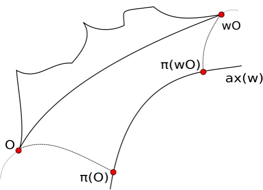
describe a quasi geodesic, therefore images of primitive elements must be loxodromic isometries. Now, fix a primitive element w and consider the situation shown in
Figure 2.2 where the curve γ is the broken geodesic which is the image under the
mapτρ,O of the path in the Cayley graph corresponding to wand readingwww . . .
O
wO
ax(w)
π(O)
[image:19.595.185.456.105.301.2]π(wO)
Figure 2.2: Projecting down the axes.
assures that the endpoints of γ and of the axes of ρ(w) coincide in the boundary at infinity. Moreover, by primitive-stability, γ is a (C, ε)-quasi-geodesic for some
uniform parameters C and ε not depending on w. This implies the existence of a
uniform constantK (depending only onC and ε) such thatγ and the axis ofρ(w) have Hausdorff distance less thanK. Consequently, there exists a constant D >0
such that if p and q are points on γ, then their hyperbolic distance is less than or
equal to the distance between their nearest point projections (onto the axes) times D, up to an additive constant. By definition of (C, ε)-quasi-geodesic, if||w||denotes
the word length ofw, then||w|| ≤CdH(O, w·O) +εfor any primitive wordw. We denote thetranslation length of an isometry S∈PSL(2,C) by l(S). Note that the
translation length and the trace of the matrix ofS are related by an explicit formula
(see Section 5.1 for the exact expression). Putting everything together we get:
||w|| ≤CdH(O, w·O) +ε≤CDl(ρ(w)) +ε.
Since there are only finitely many primitive elements with word length bounded
above by a constant, this proves that the traces of their images cannot accumulate
anywhere on the positive real semi-line.
curves on the torus, and generalisations. Extended Bowditch conditions allow prim-itive elements in F2 to have images which are parabolics in PSL(2,C). Naturally,
these representations cannot belong to PS, due to the dynamic nature of parabolic isometries. Hence we would have representations which are in the extendedBQ set but are not primitive stable. This phenomenon justifies our choice to deal only with the more classic Bowditch conditions, that give us at least one inclusion (PS ⊆ BQ) and makes the whole picture neater.
2.5.2 Two more conditions
We discuss here two sufficient conditions for primitive stability, as we shall make
use of them further on. The first result has been proved by Minsky. We just copy this specific statement here:
Proposition 2.11 ([Min], Lemma 3.2, statement (1)). Schottky characters are primitive stable.
The assumption of the proposition above can be relaxed to obtain a stronger
statement, expressed in Corollary 2.14, where we allow the character to be not purely loxodromic. The main result we need in order to prove this, is the following
proposition due to Floyd ([Flo], p.216)
Proposition 2.12 ([Flo]). Let G be a discrete, finitely generated, geometrically finite subgroup ofPSL(2,C) with no parabolics, and letO ∈H3 be a fixed basepoint.
Then there exists C >0 such that:
||g||
C ≤dH(O, g·O)≤C||g||, ∀g∈G (2.2)
If the image contains parabolic elements instead, then there existC, k >0such that:
2 log(||g||)
C −k≤dH(O, g·O)≤C||g||, ∀g∈G (2.3)
In our case we have to think of G as the image of a representation of F2. We will also need an important statement whose proof is contained in the argument
used by Minsky in [Min], Theorem 4.1:
Proposition 2.13. Letρbe discrete and geometrically finite, and letN =H3/ρ(F2)
Proof. See proof of Theorem 4.1 in [Min] for a proof of the statement.
Theorem 4.1 in [Min] assumes that the quotient manifold has a unique
block-ing cusp, but in reality the same argument is valid even when the cusps are more than one. This is further discussed in Remark 6.9 later on in the thesis.
The proof of the next corollary follows the line of Floyd’s proof of
Proposi-tion 2.12, and makes use of ProposiProposi-tion 2.13 above, extending the result stated in Proposition 2.11.
Corollary 2.14. Let ρ be discrete, geometrically finite and such that the only parabolic elements, if any, are blocking. Thenρ is primitive stable.
Proof. First of all, note that, for any pair of elements in the free group w1, w2, we have:
dH(ρ(w1)·O, ρ(w2)·O) =dH(O, ρ(w
−1
1 w2)·O).
If there were no parabolic elements in the group, then the inequalities (2.2) would
give us the desired result with g = ρ(w−11w2), but a priori only (2.3) holds. We claim that the left hand side inequality in (2.3) can be replaced with the stronger
left hand side inequality in (2.2) if we only consider words which are primitive.
Let D be a finite sided fundamental polyhedron for the group G = ρ(F2), and denote byN the hyperbolic convex hull of the limit set. LetK be the compact
set containing all geodesics corresponding to primitive elements in the quotient
manifold, as in Proposition 2.13, and let ˆK be its lift in H3. For a positive value
ε, call Mthin(ε) the ε-thin part of the quotient, that is the set of points where the injectivity radius is smaller thanε. Call H=Hε its lift to the universal cover. We
fix a value ofεsmall enough to guarantee that:
• H is aG-invariant set of disjoint horoballs, and
• H ∩Kˆ =∅.
We shall only consider the complement V = H3 \ H. Assume, without loss of
generality, that the origin O belongs to the intersection between D and ˆK. Set D0=D∩Kˆ. SinceD0 is compact, its diameter dis finite. Set
L= max
w∈F2
{||w|| |dH(O, ρ(w)·O)<1 + 2d}.
Now, take a g ∈ G which is not blocking, and subdivide the segment between O
and g·O into intervals of length 1, allowing the last interval to be shorter. Join
line between O and g·O is all contained in D0. For, g being non blocking, we
can extend it on the right to a minimal primitive word, say gp. The axis of gp
lies in ˆK, since geodesics corresponding to primitive words cannot exit the compact
set K. By Proposition 2.13, the broken line joining the closest orbit points lies
uniformly close to the axis of gp, and so does the segment [O, g ·O]. It follows
that all the segment we are considering lies in ˆK, and never intersects the set H.
The joining lines from the division points to the origin orbit travel from one copy
of D0 to the adjacent one: thus they must all have length less than or equal to 2d. Consequently, when moving from a division point to the next one along the
geodesic segment between O and g·O, then along the joining line to the closest
point in the orbit of the origin, and finally back to the geodesic line along the same joining segment, we never travel for a distance greater then 1 + 2d. It follows that
||g|| ≤dH(O,g·O)·L+ 1, giving the required inequality forg. Suppose thatw1 andw2 are primitive words inF2. Since the Cayley graph of a free group is a tree, any two of its vertices can be joined by a unique path. Suppose, without loss of generality,
that w1 = e1. . . en and w2 = e1. . . enen+1. . . en+h, where ei ∈ {a, b, A, B}. Then
w1−1w2 = en+1. . . en+h, and in particular is a subword of w2, hence not blocking, hence not parabolic. Settingg=ρ(w−11w2) we get our result.
Many conjectures have been made regarding possible relations between
prim-itive stability and Bowditch conditions.
Bowditch conjectured that in the slice of type preserving representations (i.e. characters such thattr(ρ(abAB)) =−2), BQ conditions hold if and only if the
representation is quasi Fuchsian.
As we have shown, it is easily seen that PS ⊆ BQ. Whether the two sets actually coincide is another open conjecture. In what follows, we obtain partial
Chapter 3
Primitive stability and
tessellations of the hyperbolic
plane
It is well known that the subgroup PSL(2,R) ⊆ PSL(2,C) can be identified with
the (orientation preserving) isometries of the hyperbolic plane. When the image
of a representation ρ is contained in PSL(2,R), primitive stability can be proven
by some more concrete machinery, since the geometry of the hyperbolic disc allows more “bare hands” constructions than the geometry of the three dimensional
hy-perbolic space.
Suppose for a moment that we are given a representationρ:F2→PSL(2,R) which
is discrete (in this case we say thatρ(F2) is a Fuchsian group), so that, in partic-ular, the quotient of the hyperbolic plane under the action ofρ(F2) is a hyperbolic orbifold. By classic results, one can always find a finite-sided fundamental domain
for the action of G = ρ(F2), that is a finite-sided polygon that contains exactly
one representative for each orbit. The copies of this region under the action of G
tessellate the entire plane, leaving no gaps and never overlapping. Of course, the situation changes as soon as the representation ceases to be discrete, and primitive
stability does not always hold. In what follows, we will show that, in order to prove primitive stability for a given representation, we can still proceed by similar
argu-ments. The main idea is that some property of the commutator matrix will allow
us to find some “special” polygon which will play the same role as the fundamental domain; as we act by primitive words on this region, we lay down copies of it in a
“non-chaotic” manner, without overlapping or zig-zagging too much. The precise
Remark 3.1. The techniques explained below are developed “ad-hoc” for subgroups of PSL(2,R), since the geometry of the hyperbolic plane is easier to understand
than that of the hyperbolic space. Nevertheless, the results presented in this chapter extend obviously to any group inPSL(2,C)which can be conjugated intoPSL(2,R).
We shall see that in most of the situations that we will deal with, this will indeed be the case.
We say thatρ:F2 →PSL(2,R) is a representation with intersecting axes if
the images of a pair of generators (hence any) are hyperbolic isometries whose axes
are distinct and cross. IfS, T ∈PSL(2,R), [S, T] =ST S−1T−1 encodes information
about the geometry of the elementsS andT. For a fixed representationρ, we denote byτ =τ(ρ) the trace of the matrix corresponding to the commutator of a generating
pair. The following lemma is stated and proved in [Mat] (Lemma 3.2.2).
Lemma 3.2. Suppose thatSandT are hyperbolic isometries of the hyperbolic plane, and denote by ax(S), ax(T) their axes. Suppose also that their axes are distinct. Thenax(S)∩ax(T)=6 ∅ if and only if τ =tr([S, T])<2.
Corollary 3.3. If a pair of generators has crossing axes, then so does any other pair
In other words, ρ is a representation with intersecting axes if and only if τ(ρ)<2. The restrictionτ ∈(−∞,2) still allows the commutator to be hyperbolic
(τ ∈(−∞,−2)), parabolic (τ =−2) and elliptic (τ ∈(−2,2)). In the first two cases,
the representation is discrete ([Gil]), and therefore we are in the case described in Corollary 2.14, andρis primitive stable. If the commutator is elliptic, the
represen-tation might or might not be discrete. In [Gil], the author describes a complicated
algorithm and gives a precise criterion to understand how the geometry ofρ(a) and ρ(b) determines the discreteness of the representation.
Regardless of discreteness, in this chapter we prove the following proposition:
Proposition 3.4. Letρ:F2 →PSL(2,R)be a representation with intersecting axes.
Thenρ is primitive stable.
In what follows, for simplicity, we will writeA = ρ(a) and B =ρ(b), using
capital letters for matrices, or isometries, inPSL(2,R), when no confusion can arise.
Below we give a proof of our main statement. The idea is roughly the following:
a representation with intersecting axes is always a holonomy of some geometrical
embedded polygon with side-pairings which bounds a disc in the hyperbolic plane.
When the commutator is elliptic, the polygon is a quadrilateral where opposite sides are paired by (images of) suitable generators ofF2. At this point, we use a simple
condition on the angles of this quadrilateral to carry on a geometrical argument
that concludes the proof. More precisely, we shall use primitive words to lay down adjacent copies of the quadrilateral, as one would normally do when tiling a space
with copies of a fundamental region. The simple shape of our “fundamental region”
and some observations about primitive words, will allow us to produce chains of hyperplanes (geodesics) for each broken geodesic γw arising from a primitive word
w =w(a, b). The hyperplanes will be arranged in such a way that will show that
γw is a quasi geodesic with parameters that do not depend onw, proving
primitive-stability for ρ. Let us see carefully how to do that. We have already observed that
τ has to belong to the semi-line (−∞,2) and that τ ∈(−∞,2] implies discreteness,
hence primitive stability by Corollary 2.14. We can thus assume that τ ∈ (−2,2), that is the commutator is elliptic.
Recall thatF2can be thought of as the fundamental group of a topological torus with
one open disc removed, that we denote by S11. In [Mat] (Theorem A), the author proves that a representationρ:π1(S11)→SL(2,R) is the holonomy of (at least) one
cone-manifold structure on S11 if and only if ρ is not virtually abelian. Luckily for us, virtually abelian representations cannot haveτ <2, so that representations with
intersecting axes are never virtually abelian. Therefore, our ρ induces some
cone-manifold structure onS11. It is easily seen that if the commutator is elliptic, then S1
1 with the induced structure is a torus with a unique cone-point with angle less than 2π. Following [Mat] (Lemma 5.1.5), whenever we are dealing with a holonomy
of a cone-manifold structure, we can find an immersed pentagon in H2, which is
described by the cycle:
p→B0p→A0B0p→B0−1A0B0p→[A0−1, B0−1]p→p,
where p is a generic point in H2 and if necessary we change the generating pair
(a, b) to another pair (a0, b0). Note that changing generating pairs does not affect
the geometry of a representation: the trace of the commutator is preserved under
changes of basis, so that
tr([A, B]) =tr([A0, B0]) =τ ∈(−2,2).
For this reason, with a little abuse of notation, we shall denote the new pair again
with the symbols a and b. Let p be the fixed point of the commutator. The
relation [A, B]·p = p tells us that the pentagon we had before now degenerates
to a quadrilateral with opposite sides paired by A and B and such that the sum
of the four internal angles is equal to the angle by which the commutator rotates aboutp. Also, since opposite sides are paired by isometries, and hence are of equal
lengths, opposite angles have the same amplitude, too. By [Gol2], Lemma 3.4.2, the
polygon described above is embedded, that is the four geodesic segments obtained by moving the fixed point by hyperbolic isometries are pairwise disjoint and bound
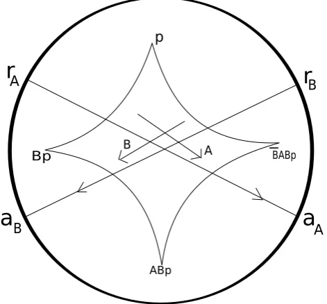
a quadrilateral. Figure 3.1 depicts the relative position of the axes, the fixed point
and the quadrilateral. Here aA, rA, aB, rB indicate the attracting and repelling
fixed points ofAand B. We can summarise the progress that has been made so far
a
a
r
r
B A
A B
p
Bp
ABp
BABp
_
[image:26.595.209.445.323.542.2]A B
Figure 3.1: The intersecting axes and the quadrilateral.
in the following way:
given a representation with intersecting axes and elliptic commutator, we can always
find an embedded quadrilateral bounding a disc in the hyperbolic plane, whose
opposite sides are paired by the isometries corresponding to a pair of generators for F2, and whose internal angles add up to the rotation angle of the commutator. Now
it is time for a little lemma:
geodesic extensions of the sides paired byB. (Clearly an equivalent statement holds by swapping the roles ofA and B.).
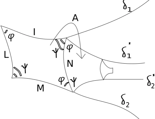
Proof. We shall use the notation shown in Figure 3.2. I,L,M, andN are the labels
I
M
L
N
A
12 1
[image:27.595.195.459.198.401.2]2
Figure 3.2: Part of the right branch of the strip of copies ofQ.
of the sides of the quadrilateral. δ1 and δ2 are the geodesics containingI andM,ϕ
andψthe internal angles at the vertices of the polygon. Consider the first adjacent
copy A·Q. The segments A·I and A·M have to lie between δ1 and δ2. For, in hyperbolic geometry the sum of the internal angles of a quadrilateral is less than
2π. Hence we immediately get
2(ϕ+ψ)<2π ⇒ϕ+ψ < π.
Moreover,δ1∩δ2 =∅, soA·I∩A·M =∅ as well. Thus the copyA·Qis entirely
contained betweenδ1 and δ2.
If we repeat the argument we see that A2·Q = A·(A·Q) is contained between
the lines δ0i =A·δi (i= 1,2). On the other hand, two geodesics can intersect only
once andδi∩δi0 is a vertex ofQ. Therefore the whole semi-line contained inδ0i and
starting fromQlies betweenδ1andδ2. This tells us thatA2·Qis not only contained
betweenδ10 andδ20, but also betweenδ1 andδ20. By repeating the argument infinitely
Now we continue with the proof of Proposition 3.4. Recall that a primitive
word inF2=ha, b|·iis an element of the group which can be extended to a minimal free generating set. As an element of F2, it can be thought of as a (cyclically
reduced) word in the alphabeta, b, a−1, b−1. We shall exploit the specific patterns
of words in F2 explained in Remark 2.2, to subdivide the word in pieces which can show a very limited number of sequences. From now on, for simplicity and
without loss of generality, we suppose that we are given a word in the lettersaand
b, w = w(a, b) = abn1abn2. . . abnp = e
1. . . en, where ei ∈ {a, b}, n = (Pini) +p.
The broken geodesicγw that we want to control is given by the sequence of vertices
. . . , e−n1p, p, e1p, e1e2p, . . .
We can label each geodesic segment inγwwith a letter, so that going alongγw reads
off. . . www . . .. As we start fromp and we move towards the “right” branch of the
line, we also lay down copies of the “fundamental polygon” Q, obtaining a strip. Going from one copy of Q to the next one, clearly reads off the same letter that
we’d read by going alongγw.
More precisely, the geodesic segment defined by the endpointsg·pandgei·p
is labeled byei. Likewise, suppose we start with a copy of the original quadrilateral,
say g·Q, and the next letter we read in w is ei. First, we bring the quadrilateral
back to the original one by applyingg−1, then we move it byei and finally we move
it back to be adjacent tog·Q. Therefore, the next copy ofQ that we lay down is
(geig−1)(g)·Q, that is gei·Q.
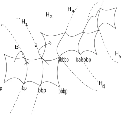
Figure 3.3 should help the reader to understand the situation. Consider the following sequence of hyperplanes. Whenever we read a b, we draw the hyperplane
given by the geodesic extending the edge between the two adjacent regions. If we find
an a, we skip that and we proceed drawing hyperplanes from the next b. Starting from p and moving forward, we also enumerate the hyperplanes as H0, H1, H2, . . ..
We claim thatHi∩Hi+1=∅ for each i.
Lemma 3.6. With the notation as above, Hi∩Hi+1=∅ for each i.
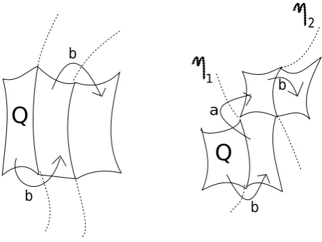
Proof. Firstly, we observe that between two consecutive hyperplanes Hi,Hi+1, we can only see two patterns: bb orbab. In the former case, the corresponding vertices
ofγw will be of the form gb·p,gbb·p, where g is some subword of a power of w. By
applying g−1, we move back to our standard configuration (shown in the left-hand side of Figure 3.4), whereQis the original quadrilateral we started from. It should
p bp
bbp
bbbp
abbbp babbbp
b a
H
3
4 5
H H
H
H
1
[image:29.595.201.443.107.337.2]2
Figure 3.3: Laying down polygons as we move along γw.
If the pattern is bab instead, then we move everything back to p as above and we are in the situation depicted in the right-hand side of Figure 3.4. Hereη1 andη2 are
just the images of Hi and Hi+1, respectively, after translating back to the origin. We claim that η1,η2 do not intersect in the hyperbolic plane, nor in its boundary. By Lemma 3.5, they should contain an infinite strip made of isometric copies of
the fundamental region, hence they cannot cross at any point in H2. If we assume
they meet at infinity, say at a pointq ∈∂H2,the situation is slightly more delicate.
Observe that η2 = ab·η1. Consider the family {lk = abkη1|k ∈ Z}. They are all
geodesic lines with one endpoint equal toq; call the other endpointqk. If
lim
k→∞qk= limk→−∞qk=q,
thenab is a parabolic element, and this gives a contradiction, since the product of
hyperbolic isometries with intersecting axes is always hyperbolic. Then, at least on
one side, lk accumulates to some limit line l. In particular, the Hausdorff distance
between lk and l goes to zero. Again by Lemma 3.5, this leads to a contradiction
since if the lines were converging, the Hausdorff distance between two consecutive
ones would become eventually less than the diameter of the quadrilateral. Thus Hi∩Hi+1 =∅ for each iand we are through.
Q
Q
b
a b
b b 1
[image:30.595.202.433.119.292.2]2
Figure 3.4: The only two possible patterns, centred at the origin.
the hyperbolic plane into two regions, one containing all theHj withj < iand one
containing all theHj withj > i. Moreover, from Lemma 3.6, the distance between
Hi and Hi+1 has to be a positive number, and this number only depends on the pattern between the hyperplanes. Since these patterns are only two, namelybband
bab, we get only two possible distances between consecutive hyperplanes. Denote byµ∈R+ the smallest among the two.
Of course we could repeat the whole story for primitive words ina−1andb, obtaining
a new valueµ0 and then choosing only the minimum between µandµ0. In this case we assume thatµis the minimum. Now, take any two vertices q1 and q2 along the
lineγw. Without loss of generality, we assume that they both belong to the positive
branch. Thus they define a subwordw0 of some power of w. Set ||w0||=n, where
||w0||denotes the usual word length in the generatorsaandb. The geodesic segment
[q1, q2] has to pass at least through n/2 hyperplanes. Split [q1, q2] in subsegments
according to the hyperplane intersection points. We see that
l[q1, q2] =dH(q1, q2)≥(
n
2 −1)µ= ( µ
2)n−µ.
Since µ does not depend on the word w, we get uniform parameters for the lower inequality for quasi-geodesics. This concludes the proof of Proposition 3.4.
one of the two is isolated. Although we do not need it here, both lemmas could be naturally extended to the more general case, dropping the isolated letter assumption.
We finish the chapter by summarising what we have proved in the following theorem, which follows by combining Proposition 3.4 with Remark 3.1.
Theorem 3.8. Let
ρ:F2 =ha, b|·i →PSL(2,C)
be a representation, and assume that there exists g∈PSL(2,C) such that
g−1ρ(F2)g⊆PSL(2,R).
Set τ =tr([ρ(a), ρ(b)]). If τ <2, then ρ∈ PS.
Observe that a group satisfying the hypotheses of the theorem above must
be made only of matrices whose trace is real, but not all groups with only real traces arise by conjugating subgroups ofPSL(2,R). In the next chapter, we shall extend
Chapter 4
Real representations,
BQ
conditions and primitive
stability
We now look at the subset of the character variety which is parametrised by triples of real numbers. A character corresponding to a triple of real numbers is called
a real representation. Throughout the chapter, therefore, each representation will be assumed to be a homomorphism ρ:F2 →PSL(2,C) such that the traces of the
image matrices of a pair of generators and their product are all real. The trace
of any other matrix in the image can be expressed as a polynomial with integer coefficients in these three traces, hence every matrix in the image must have real
trace. We try to establish a criterion under which one can decide whether a given
representation is primitive stable or not, and whether it belongs to theBQset.
4.1
Three real traces imply Fuchsian
In this section, we show that a real representation that sends generators to
loxo-dromic elements is always conjugate to a representation into PSL(2,R). A sketch
of the proof can be found in [MSW] 6.6; we present here a slightly more detailed
argument:
Proposition 4.1. Let
ρ:F2 =ha, b|·i →PSL(2,C), a7→S, b7→T.
Proof. Let us start by conjugating by an element g ∈ PSL(2,C) to put S in its
standard form:
g−1Sg= λ 0 0 λ−1
!
, λ∈R.
We now conjugate by another hyperbolic isometry h that rotates the hyperbolic
space around the axis of g−1Sg and moves one of the endpoints of g−1T g onto a real number. Write
h−1g−1T gh= u v w z
!
.
We know thattr(T) and tr(ST) are real, so that
u+z∈Rand λu+λ−1z∈R.
From the first condition we get u = x+iy and v = x0 −iy for some x, y, x0 ∈ R.
Using the second condition, we getiy(λ−λ−1)∈R. Sinceλ6=±1, it followsy = 0,
henceu, z ∈R. The fixed points of h−1g−1T gh are given by the formula
u−z±p
(trT)2−4
2w ,
and we know that at least one of the two must be real. It follows thatw, and hence
v, must be real too.
Remark 4.2. The limit set of a Fuchsian group must be contained in the equatorial circle on the Riemann sphere. If a group is conjugate to a Fuchsian group, then its limit set is again contained in some geometrical circle on the Riemann sphere. In particular, its regular set is never empty. Under this assumption, checking that a group is Schottky is equivalent to check that it is free and purely loxodromic (see Theorem 4.23 in [MT]).
4.2
The action of
Out
(
F
2)
For a given representationρ:F2 =ha, b|·i →PSL(2,C), set
x=tr(ρ(a)), y=tr(ρ(b)), z=tr(ρ(ab)).
The value of the trace of the commutator matrix depends on the three real numbers
x,y and z and can be easily computed by the polynomial identity:
We look at τ as a real function defined onR3. Clearly, a point in R3 also defines a
conjugacy class of a representation of the free group of rank 2, and identifyR3 with
the slice of the character variety corresponding to real representations.
There is a natural action of the groupOut(F2) on the character variety, defined by:
(g·ρ)(w) =ρ(g(w)).
By the observation above, the action can be though of as an action on R3, and it
is commensurable with the action of the group of automorphisms of the polynomial
4.1. This group, that we denote by Γ, is isomorphic to PGL(2,Z)n(Z2⊕Z2). In [Gol2], the author computes the generators of this group, studies its action on the
character variety and obtains some results that we shall mention below.
We let a real parameter t free to vary across the real line, and distinguish
between the following cases:
1. t∈(−∞,−2),
2. t=−2,
3. t∈(−2,2),
4. t= 2,
5. t∈(2,18], and
6. t∈(18,∞).
In what follows, we voluntarily ignore the difference between elements of the
charac-ter variety and triples of real numbers. Moreover, we shall often say just “represen-tation” instead of “class of representations”, since all the features we are interested
in are invariant under conjugation.
For each of the cases, we pick an arbitrary value oftin the interval of interest
and plot the preimageτ−1(t) or, equivalently, the zeroes of the polynomial
pt(x, y, z) =x2+y2+z2−xyz−(t+ 2).
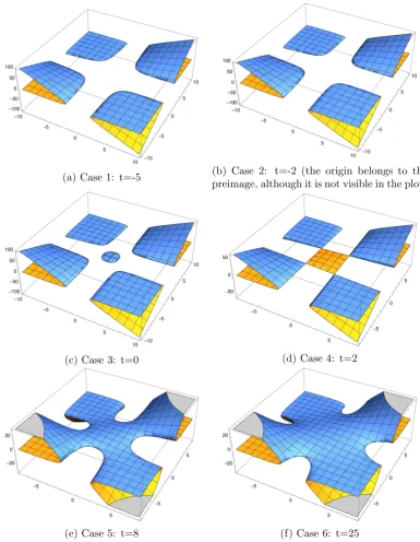
The six plots in Figure 4.1 show the behaviour of the preimage as we vary the point
in the image.
Case 1.
(a) Case 1: t=-5 (b) Case 2: t=-2 (the origin belongs to the preimage, although it is not visible in the plot)
(c) Case 3: t=0 (d) Case 4: t=2
[image:35.595.128.514.153.650.2](e) Case 5: t=8 (f) Case 6: t=25
hyperbolic structures on one-holed tori ([Gol2], §+3.2). More precisely, they can
be conjugated to Fuchsian representations which determine hyperbolic structures on one-holed tori. The commutator being loxodromic, the length of the
bound-ary geodesic is strictly positive (the exact length can be computed by Equation
5.1), therefore there are no parabolic nor elliptic elements, and by Remark 4.2 the representation is Schottky. Hence, by Proposition 2.11 or by Theorem 3.8, we
im-mediately get primitive stability and, consequently Bowditch conditions hold.
Case 2.
Here τ−1(t) is made of four copies of the Teichm¨uller space of a cusped torus and
a singular point (0,0,0). Similarly as above, points in the Teichm¨uller space corre-spond to equivalence classes of marked, complete, finite-area hyperbolic structures
on a once-punctured torus. The trace of the commutator implies that the generator
axes in the planar conjugate of the representation must cross. Again, by Theorem 3.8, we can conclude that the representation belongs to PS ∩ BQ. Observe that
here representations are not Schottky (being not purely loxodromic, thus
Proposi-tion 2.11 could not be applied). The singular point (0,0,0) is obviously outside of theBQset (and ofPS).
Case 3.
When −2 < t < 2, τ−1(t) has five connected components: one of these - call
it Ct - is compact, whereas the others are not ([Gol2], §3.3). Representations in
Ct are unitary, and unitary representations always have triples (x, y, z) such that −2< x, y, z <2 ([Gol1], Section 5) so that they cannot belong toBQ.
Alternatively, one can note that if the orbit of a representation lies in a compact, then the representation cannot be inBQby Remark 2.5. We also know that the action of
Out(F2) onCtis ergodic, and we give below (Corollary 4.5) a different proof that this
prevents the representations from being inBQ. The representations in the other four connected components can be conjugated to get characters F2 →PSL(2,R) which
give singular structures on tori with one cone point. Applying Theorem 3.8, one gets
primitive stability and belonging toBQ. Note that the elliptic commutator can have finite or infinite order. When the order is finite, the image group inPSL(2,C) is not
free. When it is infinite, the group is not discrete. However, it is never Schottky.
Case 4.
Whent= 2,τ−1(t) consists of elementary representations, which cannot be inBQ.
Here the preimage has only one connected component. Similarly to representations
in Ct from Case 3., the action of Out(F2) on τ−1(t) is ergodic for any t in this range ([Gol2], §5). According to Corollary 4.5, these representations must lie in
the complement of BQ. More concretely, one can notice that when t > 2 and the
representation is not conjugated to a Fuchsian one, by Theorem 5.2.1 in [Gol2] at least one entry in the triple (x, y, z) must belong to the interval [−2,2].
Case 6.
When t crosses the threshold t = 18, some wandering domains appear in τ−1(t).
These representations are discrete embeddings of F2 into PSL(2,C) and give rise
to complete hyperbolic structures on three-holed spheres ([Gol2], §5.1). Note that three holed spheres and one-holed tori have both fundamental group isomorphic to
F2. Let Ω0 = (−∞,−2)×(−∞,−2)×(−∞,−2) and Ω =Out(F2)·Ω0.
Ω∩τ−1(t) is the subspace ofR3 corresponding to these structures.
For representations belonging to these specific domains, once again being
Schottky assures that they belong to PS, thus toBQ.
Out(F2) acts ergodically onτ−1(t)\Ω, so the complement of Ω inτ−1(t) is made of representations which do not belong toBQby Corollary 4.5 or by the same
observation made in Case 5.
Ω⊆ R3 is the Fricke space of three-holed spheres, that is the set of points
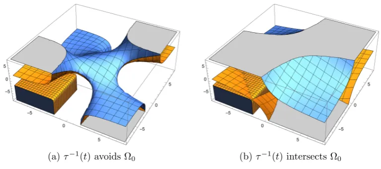
which correspond to holonomies of hyperbolic structures on three-holed spheres. As illustrated in Figure 4.1, Case 5. and Case 6. share the same preimage topological
structures. Nevertheless, as the value oft increases, the preimage surface expands
inR3 and, from t= 18 on, it starts intersecting the Fricke space. To see better how
this happens, in Figure 4.2 we plotted one component of the Fricke space (namely
Ω0) and the preimage ofτ for a value oftin Case 5 (left), and one in Case 6 (right).
The picture on the right shows a portion of the space where the surface intersects the Fricke space. Note that Ω0 is the “parallelepiped” at the left bottom corner of
both plots.
A well-known conjecture proposed by Bowditch says that if we restrict to representations with commutator trace equal to−2, then the primitive stable
rep-resentations coincide with characters satisfying theBQconditions. Another
conjec-ture claims that the whole setPS equals BQ. Neither of these conjectures, as far as the author knows, has been proved or confuted so far. The result shown in this
chapter, nevertheless, can be rephrased in the following theorem:
(a)τ−1(t) avoids Ω
[image:38.595.129.513.104.274.2]0 (b)τ−1(t) intersects Ω0
Figure 4.2: τ−1 and Ω0.
only if Bowditch conditions hold.
4.3
Ergodicity and BQ conditions
We have seen above that, when dealing with the different cases for real
representa-tions, it turns out that all the components that do not lie inBQare characterised by
an ergodic action of the group Γ. Although we did not need this information, before noticing that there was a shorter way to prove our claim, we tried to show that if
Γ acts ergodically on a component, then no element of the component can belong
toBQ. For completeness, we report here the argument that one could alternatively use, hoping that it could be useful in some more general context, when one does
not know any direct way of showing belonging to the complement ofBQ, but does
know that the action of Γ is ergodic on some connected component.
In what follows we prove that the ergodicity of the action of the mapping
class group on the character variety implies that for any open neighbourhood, al-most every point in the neighbourhood comes back to it infinitely many times.
We say that a group Γ acts ergodically on a measure space (X,A, µ) if whenever
a subset is invariant under the group action, then it has measure zero or its com-plement has. The measure µ is said to be non-atomic if for any measurable set
A∈ Awithµ(A)>0 it is possible to find a proper measurable subsetS (A, where
0< µ(S)< µ(A). In other words, µ is non-atomic if it does not admit atoms.
Proposition 4.4. Let (X,A, µ) be a measure space whereX is a topological space,
A is the σ-algebra of measurable sets in X and µ is a non-atomic measure. Let Γ
be a group acting onX, ergodically. Denote by Γ∗ = Γ\ {e}. Then for any open set
Proof. Fix any finite, positive measure setA∈ Aand define the set
EA={x∈A|Γ∗·x∩A=∅}.
We want to show thatµ(EA) = 0. First of all, we show that EA must have either
measure 0 or full measure in A. Obviously 0 ≤ µ(EA) ≤ µ(A). Suppose that
0< µ(EA)< µ(A) (note that, in particular, this implies thatµ(A\EA)>0). Then,
by ergodicity, we have that Γ·EAhas to cover the whole spaceX, up to nullsets. On
the other hand, by definition ofEA, Γ∗EA∩A=∅, hence (A\EA)∩(Γ·EA) =∅, thus
µ(A\EA) = 0, giving a contradiction. Therefore µ(EA) = 0 or µ(EA) =µ(A). We
show that the latter case cannot occur. Suppose it does occur. Then, up to nullsets,
EA=A. Pick a proper measurable subsetS (EA, with 0< µ(S)< µ(A) =µ(EA).
For the same argument as above, (Γ∗·S)∩A must have measure zero. ThusA\S
must have measure zero, contradicting the hypotheses. We conclude thatµ(EA) = 0,
as desired.
Corollary 4.5. With the same assumptions as above, if, in addition, the space X
is Lindel¨of (i.e. any open cover admits a countable subcover), then for any open set
A∈ A, for µ-almost every x∈A, the orbit Γ·x intersects A infinitely many times.
Proof. We start by defining the set
FA={x∈A| |Γ·x∩A|<∞}.
Clearly we want to show thatµ(FA) = 0. Ifx is a point in FA, then we can find a
neighbourhood Sx 3x, Sx ⊆ A, such that Γ∗x∩Sx =∅, that is x ∈ESx. By the proposition aboveµ(ESx) = 0. Now, write FA as
FA=
[
x∈FA Sx
∩FA
Since X is Lindel¨of, we can extract a countable family ofSx, say Sx1, Sx2, . . . such
that
FA⊆
[
i∈N
ESxi.
Consequently,µ(FA)<Pi∈Nµ(ESxi) = 0 and we are through.
Remark 4.6. Corollary 4.5 shows that a generic representation in a subset of R3
where Out(F2) acts ergodically is almost-surely not in BQ. Nevertheless, BQ is
Chapter 5
The diagonal slice
∆
In this chapter we introduce the diagonal slice ∆ of the character variety, that will be our main object of study for the rest of this paper. This subset, of complex
dimension one, is rich of symmetries that can be exploited. Also, the low dimension
allows us to comfortably plot pictures in the plane. We apply here some of the results obtained in the previous chapter regarding real representations. Points in
the diagonal slice that do not lie on the real line will be treated in the next chapter,
and by different techniques.
5.1
The slice and its symmetries
The diagonal slice, denoted by ∆ is defined as:
∆ ={[ρ]∈χ(F2,PSL(2,C))|trρ(a) =trρ(b) =trρ(ab)}.
In short, we are only considering the classes of representations such that both the
generators of F2 and their product are sent to matrices with the same complex traces.
Recall that the trace of a loxodromic element has an important geometric
interpretation: ifS∈PSL(2,C) is a loxodromic isometry, letax(S) denote its axis,
which is by definition the geodesic line having the two boundary fixed points ofS as
endpoints. Then there exists a complex numberl(S), called the translation length
of S, such that any point p ∈ax(S) is moved at distance <l(S) and such that the normal to the axis at the point p is twisted by =l(S). Note that l(S) is actually
traces of loxodromic elements:
l(S) = 2 cosh−1
trS 2
. (5.1)
The formula above gives us a geometrical interpretation of the diagonal slice: in
the special case of a discrete, free representation, for instance, the handlebodyH=
H3/ρ(F2) has a special 3-fold symmetry, due to the fact that the “three loops around the holes” have the same length and geometrical features. In [STY], the authors
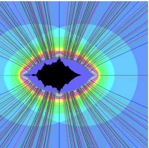
produced a very clear picture of the diagonal slice, that we are showing here in Figure 5.1. The picture represents a portion of the complex plane, where a point of complex
coordinatex is associated to the representation defined by the triple (x, x, x). The
horizontal line which runs across the picture is the real line, corresponding to real parameter triples. The setBQis the complement of the black spot in the middle of
the picture, and the complement of the ellipsoidal blue area is DF ∩∆. Although
we have good reasons to believe that the image is quite accurate in showing the set BQ, there is no theoretical proof to confirm the validity of the picture. More
precisely, the algorithm that produced the image proceeds by checking only finitely
many points, so the impression of continuity is an illusion. Moreover, for each point the algorithm performs a huge amount of computer operations to determine if the
point belongs to BQ. If certain conditions are verified during this process, then the point must belong toBQ with absolute certainty. If the conditions are not yet
satisfied after many attempts, the algorithm can only “guess” that the point does
not belong to BQ and assigns it to its complement. Hence, we know that the BQ
set could actually be bigger than what is shown in the picture.
In [STY], the authors exhibit one possible choice of generator matrices for a
conjugacy class of representations in the slice:
ρz:F2 →PSL(2,C),
ρz(a) =
9
4z2 +14 −z 2
4 + 3 4 3
4z2 −14 z 2
4 + 1 4
!
, ρz(b) = z2 4 + 1 4 − z2 4 + 3 4 3
4z2 −14 49z2 +14 !
(5.2)
The parameterz in the formulae above and the parameterx corresponding to the
“coordinate” in the complex plane shown in Figure 5.1 are related by the following
equation:
trρz(a) =trρz(b) =trρz(ab) =
9 4z2 +
z2
4 +
1
2 =x. (5.3)
|x| ≥2, then also z2 is real, and consequently the whole image of the representative character given by (5.2) sits insidePSL(2,R). In what follows, we shall say that “a
representation is Fuchsian” as a short form for “the conjugacy class corresponding to a triple contains one Fuchsian representative”.
The remaining part of this paper is devoted to showing the following main
theorem:
Theorem 5.2. Let DF be the subset of discrete and free representations. Then
DF ∩∆ is strictly contained in PS ∩∆. In particular, there exists a whole neigh-bourhood of representations in the slice which are primitive stable but do not belong toDF.
Here is an outline of the proof:
Consider ∆ as the ambient space. Points in the interior ofDF are Schottky, hence
they belong toPS by Proposition 2.11. We need to prove that every point (with a
few exceptions) in∂DF belongs toPS. Since primitive stability is an open condition ([Min], Lemma 3.2), this would immediately imply the statement of the theorem.
We shall prove that the boundary ofDF is contained in PS in the next chapter.
5.2
Real representations in
∆
Below, we consider real representations belonging to the diagonal slice. As one
can see from the picture, when restricting to real values for x, we can observe different behaviours for the corresponding representations. As usual, the main piece
of information comes from the commutator traceτ, that relates to the real parameter
xthrough
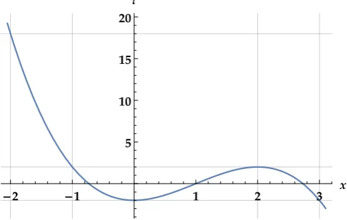
τ =τ(x) = 3x2−x3−2.
Figure 5.2 shows a plot of this polynomial function in the relevant range. The vertical and horizontal grey lines in the picture show when the function passes
through important thresholds, as discussed in Chapter 4. Note that:
τ(−2) = 18, τ(−1) = 2, τ(0) =−2, τ(2) = 2, τ(3) =−2.
Outside the plotted range, the function does not cross the horizontal stripR×[−2,2].
We organise the analysis of the real line in the diagonal slice in a short sequence of
lemmas.
Figure 5.1: A picture of the slice ∆.
Proof. This is basically Case 1 and Case 2 from Chapter 4. The representations are Fuchsian and correspond to holonomies of one holed/punctured tori.
Lemma 5.4. Representations corresponding to (2,3) are primitive stable.
Proof. This follows from Case 3 in Chapter 4, since we know that in the diagonal slice representations with real parameters with absolute value greater than or equal to 2 can always be conjugated to Fuchsian ones, hence they are not unitary. Note
that the interval (2,3) does not belong toDF, as the commutator element is always
elliptic.
When x equals 2 or −1, the commutator trace equals 2. This is the case of elementary representations, which do not belong toBQ.
For points in (−2,2), the generators are elliptic, and for x = 2 they are
parabolic, thus the representations cannot satisfy BQ conditions. Therefore:
Lemma 5.5. Representations corresponding to[−2,2]do not satisfy Bowditch con-ditions.
The only case which is left is the following: