warwick.ac.uk/lib-publications
A Thesis Submitted for the Degree of PhD at the University of Warwick
Permanent WRAP URL:
http://wrap.warwick.ac.uk/95272
Copyright and reuse:
This thesis is made available online and is protected by original copyright. Please scroll down to view the document itself.
Please refer to the repository record for this item for information to help you to cite it. Our policy information is available from the repository home page.
UNIVERSITY OF WARWICK
WMG
Fibre Reinforced
Composites via Coaxial
Electrospinning
PhD Thesis
Andrew Wooldridge 2016
Supervisors: Dr. Stuart R. Coles
i
Table of Contents
List of Tables ... iv
List of Figures ... v
List of Abbreviations ... ix
Abstract... x
Acknowledgements ... xi
Declaration ... xii
Thesis Structure ... xiii
1 Introduction ... 1
1.1 Fibres ... 1
1.2 Fibre Spinning ... 2
1.3 Electrospinning Procedure ... 4
1.4 Aims and Objectives ... 5
1.4.1 Hypotheses... 7
2 Literature Review ... 9
2.1 The History of Electrospinning ... 9
2.2 Literature Analysis ... 12
2.3 Parameter Control ... 15
2.3.1 Polymer Concentration, Molecular Weight, and Surface Tension ... 17
2.3.2 Polymer Delivery ... 20
2.3.3 Controlled Humidity ... 23
2.4 Improved Alignment and Control ... 25
2.5 Coaxial ... 29
2.5.1 Emulsion ... 32
2.5.2 Nanosprings ... 33
2.5.3 Multi-axial ... 34
2.5.4 Triaxial ... 36
2.6 High Throughput ... 40
2.6.1 Single polymer ... 40
2.6.2 Coaxial ... 42
2.7 Composites ... 43
ii
3 Experimental ... 51
3.1 General Methodology ... 51
3.1.1 Polymer solutions ... 51
3.1.2 Single Polymer Electrospinning ... 52
3.1.3 Coaxial electrospinning ... 53
3.1.4 Discussion of Parameters ... 55
3.1.5 Analytical Techniques ... 58
3.1.6 Confirmation of core-shell coaxial structure ... 61
3.2 Fibre volume fraction ... 61
3.2.1 Preparation ... 62
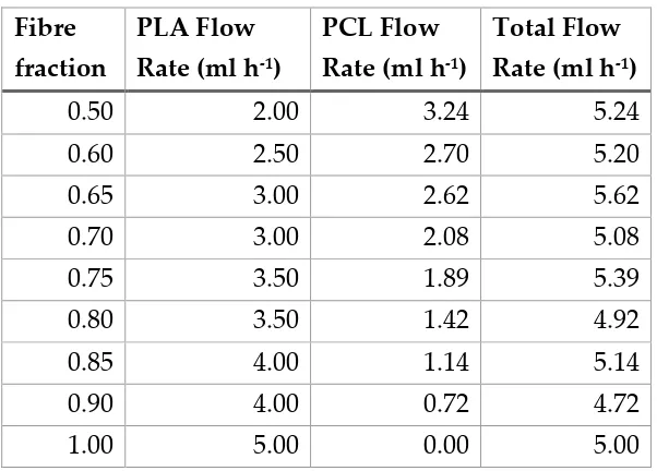
3.2.2 Electrospinning... 62
3.2.3 Composite forming ... 64
3.2.4 Materials characterisation ... 66
3.2.5 Rule of Mixtures ... 69
3.3 Composite forming variation ... 71
3.3.1 Preparation ... 72
3.3.2 Electrospinning... 73
3.3.3 Hot Pressing ... 73
3.3.4 Analysis ... 75
3.4 Coaxial and layering ... 76
3.4.1 Preparation ... 76
3.4.2 Electrospinning... 78
3.4.3 Composite forming ... 79
3.4.4 Tensile testing ... 80
4 Fibre volume fraction ... 83
4.1 Introduction ... 83
4.2 Electrospinning Polymer Fibres ... 87
4.2.1 Fibre Alignment of Electrospun Mats ... 92
4.3 Characterisation of Electrospun Fibre Mats ... 95
4.3.1 Thermogravimetric Analysis ... 95
4.3.2 1H NMR Analysis of Electrospun Mats ... 96
4.4 Tensile Testing ... 100
4.4.1 Rule of Mixtures ... 108
4.5 Conclusions ... 114
5 Composite forming variation ... 117
5.1 Introduction ... 117
5.2 Crystallinity ... 118
5.3 Tensile Properties ... 126
5.4 Fibre Deformation ... 129
iii
6 Coaxial and layering ... 134
6.1 Introduction ... 134
6.2 Electrospinning ... 134
6.3 Composite Forming ... 137
6.4 Tensile Properties ... 139
6.5 Conclusions ... 142
7 Conclusions ... 144
7.1 Fibre volume ratio ... 145
7.2 Composite forming variation ... 146
7.3 Coaxial and layering ... 148
7.4 Recommendations for Future Work ... 149
8 References ... 152
iv
List of Tables
Table 1.1: Examples of some natural and synthetic fibres. ... 2 Table 2.1: Parameters affecting the electrospinning process. Adapted from Coles et al.[51] ... 15
Table 2.2: : Concentration required to electrospin polystyrene fibres using THF.[53] .. 18
Table 3.1: Motor input voltage and corresponding collection velocity... 57 Table 3.2: Solution flow rates for electrospinning ... 64 Table 3.3: Taguchi matrix of experiments required for test the composite forming process ... 72 Table 4.1: Alignment of coaxial electrospun fibres by standard deviation from the average angle of the fibres ... 93 Table 4.2: Fibre volume fractions of composite samples analysed by NMR ... 99 Table 4.3: Actual composite test results compared to the theoretical maximum
calculated by the rule of mixtures ... 110 Table 5.1: Raw crystallinity results for the hot pressed samples ... 123 Table 5.2: Experimental variables with crystallinity and average tensile testing
v
List of Figures
Figure 1.1: Polymer dry spinning diagram ... 3 Figure 1.2: Electrospinning diagram[11] ... 5
Figure 2.1: Taylor cone visible from electrospinning polyvinyl alcohol in aqueous solution.[41] A triangle exhibting a semi vertical angle of 49.3 degrees has been
superimposed on top of the image. ... 12 Figure 2.2: The number of electrospinning papers published each year since 1995 (data adapted from Web of Knowledge) ... 13 Figure 2.3: Electrospinning research topics (data adapted from Web of Knowledge) ... 14 Figure 2.4: Samples from electrospun polystyrene, Mw = 393,400, at various
concentrations in THF.[53] ... 18
Figure 2.5: A graph showing examples of three modes of distribution. Narrow, wide, and bimodal ... 22 Figure 2.6: A graph showing how SD (%) varies with relative humidity (RH) (%) for the polymers PSU and PAN. Data adapted from Huang et al.[58] ... 24
Figure 2.7: SEM images of electrospun PSU fibres spun at different relative
humidity. (a) 0 % RH; (b) 10 % RH; (c) 30 % RH; (d) 50 % RH.[58] ... 25
Figure 2.8: Near-field electrospinning diagram[59] ... 27
Figure 2.9: Typical electrospinning instability (left), instability observed by Xin & Reneker[60] (right) ... 28
Figure 2.10: Aligned electrospun fibres produced by melt electrospinning[61] ... 29
Figure 2.11: Schematic diagram of a coaxial electrospinning spinneret (left) and pictures of a compound Taylor cone forming from a droplet (right)[62]... 30
Figure 2.12: Emulsion electrospinning. A) Nozzle setup. B) Emulsion of PMMA in PAN.[64] ... 33
Figure 2.13: Arrangements of different multi-material electrospun fibres and how they are refered to in this thesis ... 35 Figure 2.14: A multi-channel electrospinning diagram and SEM images of the
resultant fibres. Scale bars are 100 nm[67] ... 36
vi Figure 2.17: Tensile strength of glass fibres with changes in diameter. Data adapted
from Griffith.[78] ... 44
Figure 3.1: Single polymer electrospinning set-up. In this set-up the high voltage power supply is situated outside of the fume hood and is not pictured. ... 52
Figure 3.2: Coaxial electrospinning apparatus ... 54
Figure 3.3: Drawing of the coaxial spinneret (left) and the finished part (right) ... 55
Figure 3.4: Rondol bench top 10 tonne heated hydraulic press ... 65
Figure 3.5: Cooling profile of the hot press ... 66
Figure 3.6: TGA heating rate ... 67
Figure 3.7: Mini injection moulding system, Thermo Scientific HAAKE™ MiniJet Pro (left), PLA dog bone samples produced (right) ... 70
Figure 3.8: Automated hydraulic press, Collins Platen Press P 200 P/M... 74
Figure 3.9: Heating and cooling profile used during DSC analysis of the hot pressed composites ... 76
Figure 4.1: Hexagonal packing of unidirectional fibres ... 85
Figure 4.2: Schematic overview of composite forming processes for thermoplastic and thermoset matrices. Adapted from Hull[2] ... 86
Figure 4.3: PLA electrospun from a solution of 15 wt% PLA in THF (left), and from 25 wt% PLA in THF (right) ... 88
Figure 4.4: Coaxial fibres showing separation of core and shell from intentional damage. ... 90
Figure 4.5: A cross-section of coaxial fibres embedded in a matrix of PVOH. ... 91
Figure 4.6: Coaxial electrospun fibres collected at a linear drum speed of 4.87 ms-1. Yellow lines drawn on using ImageJ to calculate fibre alignment. ... 94
Figure 4.7: Coaxial electrospun fibres collected at a linear drum speed of 6.86 ms-1 .. 94
Figure 4.8: Coaxial electrospun fibres collected at a linear drum speed of 10.6 ms-1 .. 95
Figure 4.9: 1H NMR spectra for PLA dissolved in d-chloroform ... 97
Figure 4.10: 1H NMR spectra for PCL dissolved in d-chloroform ... 97
Figure 4.11: Repeating units for polymers, PLA (left), and PCL (right) ... 98
Figure 4.12: 1H NMR spectra for 0.75 fibre volume ratio composite dissolved in d-chloroform ... 98
Figure 4.13: Consolidated coaxial electrospun composites cut into 15 mm strips and labelled for tensile testing. Each square on the mat is 10 x 10 mm. ... 100
vii Figure 4.15: Typical stress-strain curves for the composites from a selection of fibre volume fractions, and compared with the bulk polymers. The bulk PCL curve
extends to 22% strain, but it has been truncated in this graph for clarity. ... 102
Figure 4.16: Young's modulus compared to volume fraction of PLA in the composite with standard deviation error. ... 103
Figure 4.17: Tensile strength compared to volume fraction of PLA in the composite with standard deviation error. ... 103
Figure 4.18: Elongation at break compared to volume fraction of PLA in the composite with standard deviation error. ... 106
Figure 4.19: A sample of tensile test results for composite samples of 0.73 volume fraction of PLA ... 107
Figure 4.20: A sample of tensile test results for composite samples of 0.92 volume fraction of PLA ... 108
Figure 4.21: Measured Young's modulus of the electrospun composites compared to the upper and lower bound calculated by the rule of mixtures... 111
Figure 4.22: Measured tensile strength of the electrospun composites compared to the upper and lower bound calculated by the rule of mixtures... 111
Figure 4.23: Cross section of a 0.56 fibre volume fraction composite showing uneven distribution of PLA fibres in the PCL matrix ... 112
Figure 4.24: Cross section of a 0.73 fibre volume fraction composite showing even distribution of PLA fibres in the PCL matrix ... 113
Figure 5.1: DSC curve of PLA as received, showing two cycles of heating ... 119
Figure 5.2: DSC curve of PCL as received, showing two heating cycles and the first cooling cycle. ... 120
Figure 5.3: DSC curve for a sample of coaxial PCL/PLA as spun, before hot pressing. ... 121
Figure 5.4: DSC curve for experiment 3, a composite pressed at 10 bar and 110 °C and cooled at 10 K/min, resulting in 27.64 % crystalline PLA. ... 125
Figure 5.5: Effect of PLA fibre crystallinity on the tensile strength of the composites ... 127
Figure 5.6: Effect of PLA fibre crystallinity on the Young's modulus of the composites ... 128
Figure 5.7: Effect of composite forming temperature on the tensile strength ... 129
Figure 5.8: Cross-section of a composite pressed at 70 °C and 1 bar ... 130
Figure 5.9: Cross-section of a composite pressed at 110 °C and 1 bar ... 130
ix
List of Abbreviations
AFM – Atomic force microscopy
CNC - Computer numeric control
CRP – Carbon fibre reinforced polymer
DMF – Dimethylformamide
DoE – Design of experiments
FPR – Fibre reinforced polymer
GRP – Glass fibre reinforced polymer
HVDC – High voltage direct current
PAN - Poly(acrylonitrile)
PCL – Polycaprolactone
PLA – Poly(lactic acid)
PP – Polypropylene
PSU – Polysulfone
PTFE – Polytetrafluoroethylene
PVOH – Polyvinyl alcohol
RH – Relative humidity
SEM – Scanning electron microscope
TEM – Transmission electron microscope
THF – Tetrahydrofuran
wt% - Weight percentage (concentration)
x
Abstract
This study shows that an all-thermoplastic (nano- or micro-fibre) polymer can be
created using coaxial electrospinning to create fibre mats akin to pre-impregnated
fabric, which can be formed into a composite without the addition of other materials.
This has not yet been accomplished by using the coaxial electrospinning production
process. Experimentation to investigate the maximum fibre volume ratio found that
these composites were successfully formed at 0.73 fibre volume fraction, which is
higher than the maximum found in traditionally formed composites (0.60 – 0.70).
The formation of the composite from the fibre mats was investigated, and found that
the composites formed at the lowest temperature and pressure (70 °C and 1 bar)
exhibited the higher tensile strength, up to 84 % higher than at other temperatures
and pressures. Higher pressure and temperature caused deformation in the
reinforcing fibres, resulting in lower tensile strength. The composites were shown to
have more consistent Young’s modulus and higher tensile strength compared to a
composite made from the same materials, but with the fibres and matrix materials
produced separately, and combined during the composite forming procedure.
The finalised composite produced in this research exhibited an average Young’s
Modulus of 2.5 GPa, ultimate tensile strength of 33.2 MPa, and elongation at break of
xi
Acknowledgements
Firstly, I would like to thank my supervisors, Dr. Stuart Coles and Professor Kerry
Kirwan, for guiding and supporting me through the PhD process.
Thank you to the University of Warwick, WMG, and all the technical staff who put
up with me and my project, and for training me and letting me use their equipment.
I am especially grateful to the EPSRC who have made this research possible through
their generous funding. Thank you to my friends and co-workers who helped to
create an enjoyable and friendly office environment.
I would also like to thank my friends and family for their support, not just during
my PhD, but everything they have done for me leading up to it. I am especially
thankful to my girlfriend, Louise, for her unconditional love and support.
Lastly, and most importantly, I would like to thank anyone reading my thesis, as this
xii
Declaration
This thesis is submitted to the University of Warwick in support of my application
for the degree of Doctor of Philosophy. I hereby declare that this thesis is my own
work and effort, and that it has not been submitted anywhere for any other award.
xiii
Thesis Structure
Chapter 2: Literature Review
This details the current and past work on the subject matter, and where this project fits in. The various capabilities and processing of
electrospinning are included here.
Chapter 4: Fibre Volume
Ratio
The results of varying the fibre volume ratio of the coaxial electrospun composite. Chapter 5: Composite Forming
The effect of the forming
temperature, pressure, and cooling rate on the tensile
properties of the composite. Chapter 6: Layering Technique A comparison between a laminate
structure of fibres and sheet matrix, and coaxial fibre-matrix mats. Chapter 3: Experimental
Experimental methods for the following three chapters. Chapter 1: Introduction
A short insight into the objectives of this project and its impact.
Chapter 7: Conclusions
1
1
Introduction
1.1
Fibres
It is difficult to find a universal definition for a fibre. ISO 8672 is a standard detailing
air quality, and defines a fibre as “any object having a maximum width less than 3 μm, an
overall length greater than 5 μm and a length to width ratio greater than 3:1”.[1] This,
however only concerns fibres hazardous to health via inhalation. In reality, the
definition of a fibre appears open to interpretation. Within composite materials
fibres can be classed as continuous (long) or discontinuous (short).[2] This thesis is
concerned with the production of continuous fibre composites.
Fibres are used in everyday life in applications such as textiles, paper, and rope.
They are used in place of bulk material due to their inherent high tensile strength.
All materials have a theoretical strength calculated from the atomic forces within
them, but in reality the strength is much lower than this due to defects and
dislocations within the structure creating weak points at which the material can
break. Fibres possess a small cross sectional area, so there is little room for defects,
resulting in higher strength than bulk material.[3]
The strength of fibres is used throughout nature in plants, animals, and minerals.
2
Table 1.1: Examples of some natural and synthetic fibres.
Natural Synthetic
Plant Animal Mineral Polymer Other
Cellulose Silk Asbestos Nylon Glass
Cotton Wool Glass* Rayon Carbon
Jute Acrylic Metallic
Hemp Polyester
Flax Aramids
*Glass fibres can (rarely) be found naturally as form of lava known as “Pele’s Hair”
Since the first synthetic polymer fibre, nylon, was produced in 1935, interest in
synthetic fibres has continued to increase due to their low cost and availability. More
recently, research has turned back to natural fibres due to the increasing cost of oil,
and the drive towards reducing carbon emissions.[4]
1.2
Fibre Spinning
Synthetic polymer fibres are usually produced from an extrusion process called
spinning. This involves pushing a viscous liquid through tiny holes of a spinneret
and solidifying the liquid into a fibre on the other side. The different processes that
can be used are: wet spinning, dry spinning, melt spinning, and electrospinning.[5,6]
Wet and dry spinning both use a polymer dissolved in a solvent to form a solution.
In wet spinning the solution is pushed through the spinneret into a chemical bath
where the polymer is precipitated out to form a fibre; whereas in dry spinning, air
flow is used to evaporate the solvent to solidify the polymer. Melt spinning can be
3 cooled after being pushed through a spinneret. In gel spinning the polymer use is of
high molecular weight resulting in a highly viscous solution. This draws out and
aligns the polymer chains, increasing the strength of the fibres. Typically, after each
of these types of extrusion, post processing of the fibres is carried out to wash and
dry the fibres. They are then drawn out to increase strength and orientation of
molecular structure.
Figure 1.1 shows a diagram of a basic spinning process. It could be modified to
[image:18.595.192.399.348.590.2]include a chemical bath for wet spinning; or an air flow for dry or melt spinning.
Figure 1.1: Polymer dry spinning diagram
Compared to these more conventional techniques, electrospinning is a differs in that
the polymer fibre is drawn out of a solution, or melt, using electrostatic force.
4 Compared to other spinning techniques, electrospinning can manufacture thinner
fibres, ranging from 10 μm to 10 nm.[7]
1.3
Electrospinning Procedure
In a typical modern electrospinning set-up,[8] a droplet of viscous polymer solution,
or melt, held on the tip of a needle or nozzle is charged by using a high voltage
direct current (HVDC) power supply, typically between 5–20 kV. The polymer can
be fed to the needle either using a gravity feed or a syringe pump to ensure a
constant droplet is formed. The electric charge causes the droplet to deform, creating
a Taylor cone. This is a perfect cone with a semi-vertical angle on 49.3 ° just before it
reaches a critical voltage where the electrostatic force overcomes the surface tension
of the polymer, ejecting a thin jet from the tip. The jet stretches out and enters an
unstable region where it whips about due to the repulsion of charge, which stretches
the jet and evaporating the solvent, or cooling the melt. The solid fibre can then be
collected onto a grounded or oppositely charged collector. This process is
represented in the labelled diagram in Figure 1.2. The collector can either be a
stationary plate, in which case the fibres collected will be randomly aligned, or onto
a rotating collector, which, if it is rotating at the same speed as the jet is being
collected, the fibres will all be aligned in one uniform direction. This rotation speed
can vary between a large range of values; for example, Sundaray et al.[9] observed
that while electrospinning poly(methyl methacrylate) (PMMA) and polystyrene (PS)
5 whereas Fennessey and Farris[10] reported optimal fibre alignment when using
[image:20.595.98.495.145.373.2]collection speeds of 8.1 to 9.8 ms-1.
Figure 1.2: Electrospinning diagram[11]
1.4
Aims and Objectives
This thesis looks into a novel methodology for creating fibre-reinforced composites
using a coaxial electrospinning technique. The literature review has shown that there
is a wealth of electrospinning papers, with the numbers increasing every year. There
is currently limited research which looks into the use of electrospun polymer fibres
in composite materials, and no research on using coaxial techniques to produce a
fibre mat suitable to form a fibre reinforced composite in a one step process of
applying heat and pressure. The aim of this thesis is to address that gap.
In order to achieve this, the following objectives have been set:
6
• Optimise the technique to improve the tensile properties of the composite
• Investigate and compare the performance of the coaxial electrospun
composite
The polymers being used are poly(lactic acid) and polycaprolactone; both of these
are biodegradable and biocompatible. These polymers have been chosen due to both
these qualities and also their thermal and mechanical properties. The biodegradable
and biocompatible nature of the polymers allows the finished composite to be used
within the body for soft tissue reinforcement, and the thermal and mechanical
properties ensure that the composite can be successfully formed.
Soft tissues within the body can be damaged through everyday wear and tear, and
also from accidental injury; particularly when doing sports. Torn tendons and
ligaments can be stitched together during surgery, but the result is a weak
connection which can easily be subject to further injury before healing has
completed.
Various materials can be used to reinforce where the soft tissues have been joined to
both take some stress off the stitches, and to cover the soft tissue to prevent abrasive
damage. Commercial products currently include reinforcement constructed from
human tissue,[12] animal tissue,[13] and synthetic polymers.[14]
Muscle tendons are long fibrous structures,[15] similar, in a fashion, to an aligned,
7 tendons have shown that, depending on the location within the body, and age of the
person, they can have a Young’s modulus from 0.6– 2 GPa, ultimate tensile strength
from 4 - 100 MPa, and 3 – 10 % elongation at break.[15–18] If the composites produced
in this work are to be used as a tendon reinforcement, these values will need to be
exceeded, or at least matched.
1.4.1
Hypotheses
It is expected that the composites formed from the coaxial electrospun fibres will be
heavily affected by small changes in the production process. In order to improve the
tensile properties of the composite, both the electrospinning process and the
moulding process will be varied. By varying the electrospinning process, the fibre
volume ratio of the composite can be altered. Literature suggests that for this type of
composite, fractions between 0.6 and 0.7 are usually considered to be the maximum
due to uneven distribution of fibres and imperfect wetting of the fibres by the
matrix.[2] This is further discussed in section 2.7. It is expected that the coaxial
electrospun fibre composites will be able to challenge this, and produce successful
composites with similar or higher fibre volume fractions.
Composite forming is commonly conducted under compression and vacuum
moulding. The pressure exerted from vacuum moulding is restricted to one bar
(atmospheric pressure), whereas the pressures from compression moulding are
much higher, but can be more expensive to run. It is expected that the higher
8 higher tensile properties by reducing voids and facilitating better fibre to matrix
adhesion. Although higher moulding temperatures will reduce the viscosity of the
molten PCL matrix, the PLA fibres have a low glass transition temperature and the
heat combined with the pressure could deform the fibres. There is also the possibility
that the crystallinity of the PLA fibres could be increased by pressing at a higher
temperature, as it can undergo cold crystallisation from 90 -100 °C.[19] A change in
crystallinity can affect the tensile strength and Young’s modulus of the fibres, and
therefore, the composite.[20] Composites with different tensile properties could be
produced from either a lower temperature forming process just above the melting
point of PCL, and a higher temperature process to encourage the crystallisation of
PLA.
The coaxial fibres are structured so that low penetration of the matrix material
through the fibres is needed, as the material is already dispersed throughout them.
This counteracts the main disadvantage of the high viscosity of a thermoplastic
compared to a thermoset, as the matrix material is already in place. It is expected
that this placement of the matrix will result in a better performing composite,
compared to one formed using the same conditions as the coaxial fibres, but with the
9
2
Literature Review
2.1
The History of Electrospinning
The effect of electricity on fluids was realised before electricity was even fully
understood. This began in 1600, when William Gilbert observed that a droplet of
liquid could be deformed into a cone shape (now known as a Taylor cone) using a
piece of charged amber. However, a stream or jet of ejected particles was not noted
until 1750 by Jean-Antoine Nollet, who realised a charged droplet would eject a
spray if near an electrical ground. This is thought to be the first reference to
electrospraying, the precursor to electrospinning, where the conditions are not
suitable for electrospinning (such as the viscosity of the liquid being too low), and
the jet breaks up into droplets due to the Rayleigh instability.
Electrospinning was first documented in 1887 by C. V. Boys.[21] He refers to it as “the
old, but now apparently little-known experiment of electrical spinning”, and made the
observation that when the solution was viscous and expelled at high voltage it
became a fibre, but as the liquid was heated and became less viscous, the jets broke
up into droplets, as in electrospraying.
The first British patent for electrospinning was issued in May 1900 to J.F. Cooley,[22]
and the first US patents issued in February 1902 to J.F. Cooley[23] and in July 1902 to
W.J. Morton.[24] In these patents, Cooley specified a number of different nozzle
10 around the polymer, slowing down the evaporation of the solvent and the
solidification of the polymer.
The first attempt to mathematically model the electrostatic deformation of liquids
was by John Zeleny who published a number of papers from 1907 to 1920.[25–29] He
investigated how the liquids behaved under various voltages from different
electrodes, determining that the diameter rather than the shape of the electrode
affected the discharge. His experiments with different voltages also showed the
change in shape of the droplet as the voltage increased, the stability of the current
flow over these voltages, and how it varied from being steady to unstable and steady
again as the voltage increased.[26]
Electrospinning patents continued to be filed, with Anton Formhals being issued 10
electrospinning patents in the United States of America, and 22 worldwide[30] from
1931 to 1944. In his patents, Formhals mainly focused on variations of the
electrospinning set-up and using them to produces textiles and yarns. His inventions
included different collection methods; such as, on rotating belts[31–35] and between
charged wires,[36] and different charging methods; charging the nozzle and the
collector,[31–35,37–39] and only charging the collector.[36]
In 1938 in Russia, Igor Vasil’evich Petryanov-Sokolov and Natalya D. Rosenblum
produced fibres from cellulose acetate from which they developed a filter, known as
a “Petryanov filter”. A factory producing these filters was established, producing
11
were used in the “Lepestok” particulate filter mask in the nuclear industry. Five
billion units were produced by 2003 and they are still commercially available
today.[30] These filters have been claimed by the source to be the first commercial
usage of electrospun fibres.
In 1964, Sir Geoffrey Ingram Taylor started to look at the deformation of liquid
droplets in more detail. He built on Zeleny’s work from earlier in the century;
applying corrections to the work and implementing his own theories. Taylor
theorised that when a droplet was extended to 1.9 times its equatorial diameter it
would become unstable, developing a conical point which would project jets of the
fluid. He derived that the cone would exist in equilibrium with a semi-vertical angle
of 49.3°, and showed experimentally that the cone would expel jets of liquid as it
neared this value.[40] This cone, formed from a fluid droplet under the influence of an
electric field, is now known as a Taylor cone. Figure 2.1 shows a Taylor cone formed
from electrospinning a solution of polyvinyl alcohol. A triangle with a semi vertical
angle of 49.3 degrees has been drawn on top of the image to visualise Taylor’s
12
Figure 2.1: Taylor cone visible from electrospinning polyvinyl alcohol in aqueous solution.[41] A triangle exhibting
a semi vertical angle of 49.3 degrees has been superimposed on top of the image.
Interest in electrospinning halted for a time, as few applications could be identified.
However, advances in nanomaterials in the 1980s and 1990s once again sparked
interest into the potential uses for electrospun fibres. The modern age of
electrospinning began in 1995, with the publication of the Doshi & Reneker paper[42]
which popularised the term “electrospinning” for the process; previously known as
either electrical or electrostatic spinning.
2.2
Literature Analysis
Since the dawn of modern electrospinning research in 1995, studies into this field
have gathered more interest every year. This is evidenced by the increasing number
13
Figure 2.2: The number of electrospinning papers published each year since 1995 (data adapted from Web of Knowledge)
Electrospinning is a versatile process with a lot of scope. Although more demanding
to replicate on an industrial scale, a basic laboratory set-up for research can be
relatively cheap and simple. The process of electrospinning is quite sensitive and can
be difficult to control, as minor changes in the parameters can affect the resulting
fibres. As a result of this, and the inexpensive cost, many papers are published
merely detailing the successful electrospinning parameters and investigating the
subsequent morphology of the resulting fibres. A 2005 study[20] showed that 60 % of
electrospinning research was on processing and characterisation of electrospun
fibres. A Web of Knowledge search shows that more recently this number has
dropped to 30 % as shown in Figure 2.3. This could be due to a shift from the
0 500 1000 1500 2000 2500 3000
19
95 1996 1997 1998 1999 2000 2001 2002 2003 2004 0520 2006 2007 2008 2009 1020 2011 2012 2013 2014 2015
Num
b
er
o
f
pa
pe
rs
pub
li
sh
ed
14 exploration of the fundamental principles to the consideration of material properties
[image:29.595.116.522.150.443.2]and applications.
Figure 2.3: Electrospinning research topics (data adapted from Web of Knowledge)
The largest area studied appears to be in the biomedical field, where many uses have
been found due to the ease of fabricating biocompatible polymers with large surface
areas. The small batch, customisable production of electrospinning also fits well
within this niche area due to requirements for bespoke applications within the body.
Research is on-going using electrospun fibres for drug delivery,[43] wound
dressing,[44–46] and bone scaffolds.[47,48]
The second largest area with regards to applications is within electronics as recently
there has been a surge of interest in alternative energy; as electrospun fibres have
Biomedical 30%
Characterisation 25% Electronics
14% Mechanical
Strength 11% Fabrication
5% Sensing
3%
Filtration
15 been shown to be of use as membranes in fuel cells,[49] and as electrodes in lithium
ion batteries.[50]
2.3
Parameter Control
Although the research into characterisation and fabrication is slowing down, it
remains relevant as it provides an understanding of the fundamentals of the process.
At the forefront of this is the control of the parameters, which can be grouped into
solution, process, or environmental, as shown in Table 2.1. Some of the
environmental parameters involved affect the process by modifying the others. For
example, an increase in temperature can decrease the viscosity of the solution, and a
decrease in pressure will cause the solvent to become more volatile.
Table 2.1: Parameters affecting the electrospinning process. Adapted from Coles et al.[51]
Solution parameters Process parameters Environmental parameters
Concentration Electrostatic potential Temperature
Viscosity Electric field strength Humidity
Surface tension Electrostatic field shape Local atmosphere flow
Conductivity Working distance Atmospheric composition
Dielectric constant Feed rate Pressure
Solvent volatility Orifice diameter
The successful production of fibres from electrospinning requires a careful balance
of the parameters involved.[52] For example, if the spinning voltage is increased the
polymer will be ejected more rapidly from the spinneret, therefore the polymer feed
16 to the collector is increased, the voltage would also have to be amplified to maintain
the electric field strength, in order for the polymer strands to be ejected. These
limiting conditions were realised in the first documented electrospinning
experiment:
“The conditions for the success of this beautiful experiment are not very easily obtained”
-C.V. Boys, 1887[21]
This encourages researchers to investigate additional control measures to stabilise
the process, and offers a way to alter the properties and morphology of the resulting
fibres whilst keeping the input material constant. The production of smooth,
consistent electrospun fibres is important in a wide range of applications. A
homogenous mat ensures even pore size, important for use as a filter; mechanical
strength, for general use and especially as reinforcement in composites; and an even
surface area across the mat, for biomedical uses such as drug delivery and cell
scaffolds.
Coles et al.[51]conducted a design of experiments (DoE) to investigate the effect of
variables on the fibre output of polymers polylactic acid and poly(vinyl alcohol). The
variables examined were: conductivity with the addition of salt, concentration,
electrostatic potential, and the collection distance. It was concluded that the
interactions between the variables had a great effect on the output fibres and
material properties, which were able to vary diameters from 0.16 to 5.29 μm, and the
17 This was a simple experiment demonstrating the ease at which a single variation in
the experimental setup can have a profound effect on the fibres produced.
The following sections details some of the parameters which have the greatest effect
on the outcome and success of the electrospinning process. Firstly, the parameters of
the polymer solution will be discussed, which can determine whether a fibre can be
produced. This will be followed by variations in which the polymer can be
delivered, and finally how variation in humidity can affect the surface of the
electrospun fibres, introducing roughness and pores.
2.3.1
Polymer Concentration, Molecular Weight, and Surface
Tension
As the concentration and molecular weight of a polymer in solution increases, the
viscosity of the solution increases. This is because of the nature of the polymer
chains; as the longer chains, or higher concentration of chains increases, the
interactions between then increase in the form of the Van de Waals forces and chain
entanglement.[20] This is an important parameter in forming the fibres during
electrospinning.
Eda & Shivkumar[53] experimented with varying the concentration of polystyrene
dissolved in tetrahydrofuran and dimethylformamide, for a variety of different
molecular weights. Using polystyrene at Mw= 393,400 g mol-1 it was observed that for
18 fibres are visible connecting the beads, and at 18.9 wt% the polymer transitions to a
bead on a string structure. At 21.2 wt% smooth fibres are formed with no beading.
SEM images of these results are shown in Figure 2.4.
Figure 2.4: Samples from electrospun polystyrene, Mw = 393,400, at various concentrations in THF.[53]
The same pattern was observed for all molecular weights tested, however the critical
concentration at which the smooth fibres were formed decreased as molecular
weight increased and vice versa. Table 2.2 shows the finding for the critical
[image:33.595.124.471.178.434.2]concentration for each molecular weight tested.
Table 2.2: : Concentration required to electrospin polystyrene fibres using THF.[53]
Molecular Weight (g mol-1)
19,300 44,100 111,400 393,400 1,045,000 1,877,000
Critical
Concentration (wt%)
19 These results imply that the effect of both the molecular weight and concentration
have on the viscosity are the main factors in forming the fibres, rather than the
variables themselves, and as expected critical concentration decreases as viscosity
increases. Further work could be done to investigate the viscosity of the solutions at
the critical concentrations for each molecular weight.
Yang et al.[54] performed similar work investigating the influence of solvent on
electrospinning poly(vinyl pyrrolidine). They reported the same findings as Eda &
Shivkumar[53] for low concentrations of polymer in solution producing the bead on a
string morphology. In addition, they found that a further increase of concentration
caused the average fibre diameter to increase from 120 nm to 1.5 μm for
concentrations of 2 wt% to 10 wt%. At 20 wt% it was observed that the fibres formed
a helical pattern on the collector resulting from the bending instability of the process.
The process was unsuccessful from 25 wt% as the viscosity of the solution was too
high.
Yang et al.[54] also investigated the effect of surface tension on the electrospinning
process by dissolving the polymer in different solvents, and by using a mix of
solvents. The solvents used were: dimethylformamide (DMF), dichloromethane
(DCM), and ethanol. It was found for the solutions with low surface tension, using
ethanol, smooth fibres were produced, but with high surface tension, using DMF,
20 These beading effects are due to fluid thread breakup which causes the jet to divide
up into droplets. In electrospraying, this effect is taken advantage of, but in
electrospinning everything is done to prevent this from happening. The rate at
which a viscous fluid thread is broken up into droplets is governed by equation (2.1),
derived by Rayleigh in 1892:[55]
𝑖𝑛 = 𝝈
6𝑎𝝁 (2.1)
In this equation σ is the surface tension of the fluid, μ is the viscosity of the fluid, a is
the initial radius of the fluid jet, and in is the growth rate of the instability. The
equation shows that increased viscosity and decreased surface tension will each slow
the rate at which the thread is broken up into droplets. This results in less beading
and smoother fibres being produced from electrospinning.
2.3.2
Polymer Delivery
A challenge which may be faced when electrospinning is to keep the polymer
droplet a constant size and shape, in order to protect the stability of the jet. This
ensures that the fibres deposited on the collector are of a consistent diameter, an
advantage in almost all applications. This is usually done by using a syringe pump
set to a constant flow rate to match the rate at which the polymer is ejected. Some
researchers have attempted to ensure a stable droplet by using feedback control,
21 of using cameras to measure the volume of the droplet, and measuring the current
across the jet to keep it constant.[56]
Druesedow et al.[56] used an elaborate setup of pneumatics and pressure control
devices to achieve a constant droplet. The syringe pump pumps air into a bottle
containing polymer solution, which is ejected out of the bottom through a needle.
The pressure control system employs sensors to measure the air pressure inside the
bottle, and the height of the polymer solution. Two methods for measuring the level
of the solution were tested: infrared, and ultrasonic. Both of these methods appear to
have their advantages and disadvantages. The infrared method is a cheaper solution,
but is intrusive, as a float has to be employed on the surface of the polymer solution
to get an accurate measurement. A number of drips were also observed with this
method. The ultrasonic transducer, however, was non-intrusive, but more expensive
and more sensitive to disturbances. However, no drips were observed. Despite the
poorer performance of the infrared sensor, both methods appeared to produce fibre
mats similar in fibre density and morphology (500 - 850 nm), and the diameter of the
fibres was easily controlled by adjusting the pressure of the system.
This report, however, does not comment on a comparison with a fibre mat spun
without any feedback control, and no detailed information is given about the spread
data. Although a rough range of data is presented, the standard deviation of the
fibre diameters calculated from a representative sample would provide better
22 distribution of fibre diameters might appear. The narrow distribution is preferable
when trying to create the most consistent fibres in the mat as the range of fibres is
contained. The wide distribution represents a sample without consistent fibre
diameters, and the bimodal distribution characterises a sample in which the fibres
diameters converge upon two points. This shows that there may be few fibres
measuring around the mean values, and without more information it is impossible
to know the reliability of the data presented.
Figure 2.5: A graph showing examples of three modes of distribution. Narrow, wide, and bimodal
The quality of electrospinning results can vary widely, so without a proper
comparison with the more traditional method of using a constant flow rate the
experiment has not proven that its more elaborate set-up is necessarily
advantageous. It does, however, successfully offer a different approach to delivering
the polymer solution which may be valuable if traditional methods are unsuccessful.
F
re
q
u
en
cy
Fibre diameter
Narrow
Wide
23
2.3.3
Controlled Humidity
Varying the humidity during electrospinning can introduce pores onto the surface of
the fibres. In dry conditions smooth fibres can be produced, but as humidity
increases, as does pore frequency and size (diameter and depth).[57] Controlling the
humidity is one of the simplest ways to control the surface of electrospun fibres as it
remains a one-step process as no post processing is required.
Huang et al.[58] performed humidity control while electrospinning poly(acrylonitrile)
(PAN) and polysulfone (PSU), each dissolved in DMF. The morphology and
mechanical strength was investigated as the relative humidity (RH) was increased in
10 % increments from 0 %. The PSU fibres appeared to be affected by a greater
degree than the PAN fibres by the changes in RH, as pores were formed on the PSU
fibres, but the PAN fibre only exhibited increased surface roughness. This is
attributed to PSU being hydrophobic, and PAN being hydrophilic, so the moisture
on the PSU will form droplets on the surface, leaving indentations (pores). Figure 2.7
shows detailed SEM images of some of the PSU fibres produced with visible pores.
Electrospinning at high humidity was unsuccessful as no fibres could be produced
after 50 % for PSU and 60 % for PAN.
As the RH increased a steady increase in the average diameter of the fibres was
observed, from 1.15 μm to 3.58μm for PSU and from 150 nm to 630 nm for PAN,
with the standard deviation (SD) peaking at the low and high humidity values, as
24
Figure 2.6: A graph showing how SD (%) varies with relative humidity (RH) (%) for the polymers PSU and PAN. Data adapted from Huang et al.[58]
Both polymers appear to have a point where mechanical strength increases with
humidity, but quickly drops as humidity further increases. For the PAN this appears
at 20 % RH and for the PSU at 10 % RH. The electrospun fibres were only being
collected at 70 RPM, which appears to be slower than the deposition rate of the fibre,
as the mats produced are not aligned. As a result, the adhesion between the fibres
will be a main contributor to the tensile properties of the mat. It is theorised in the
paper that the high humidity results in phase separation causing a skin to form on
the surface of the jet, and resulting in weaker fibre to fibre adhesion in the mat,
causing the decrease in strength at high RH.
0 10 20 30 40 50 60 70 80 90
0 10 20 30 40 50 60 70
25
Figure 2.7: SEM images of electrospun PSU fibres spun at different relative humidity. (a) 0 % RH; (b) 10 % RH; (c) 30 % RH; (d) 50 % RH.[58]
Controlling atmospheric conditions is difficult without the correct equipment, but it
is clear that it can affect the results of the electrospinning process enormously.
Further experimentation could be conducted to investigate the effects of humidity on
the mechanical strength of aligned fibres.
2.4
Improved Alignment and Control
In some applications, such as composites, the alignment of the fibres plays an
important role in the performance of the product. Using a rotating mandrel to collect
26 on the speed of the mandrel. While this method is satisfactory for most applications,
it is possible to produce accurately aligned fibres by removing the instability portion
of the electrospinning process; either by reducing the collection distance so that the
fibre does not have a chance to enter this instability,[59] or by adjusting the voltage to
a point where there is an instability at the beginning of the jet, but the coils shrink,
and the jet becomes straight again.[60] This manipulation of the jet can allow for the
controlled deposition of the polymer fibre making it possible for it to be used in a
similar fashion to a printer. Reducing the bending instability, however, means that
the fibre may not stretch as much, and will be thicker.
Sun et al.[59] used a short collection distance, with a tungsten electrode with a 25 μm
tip to construct fibres 50-500 nm in diameter. Unlike a conventional electrospinning
set-up, the polymer solution is applied to the tip of the electrode by dipping it in the
solution prior to the spinning. This, however, presents the disadvantage of not being
able to produce a continuous jet. Concentrations of solution from 3 - 5 wt% of
poly(ethylene oxide) were used. The experiment was successful with the minimum
spinning voltage at 600 V, and the minimum collection distance 0.5 mm. Figure 2.8
27
Figure 2.8: Near-field electrospinning diagram[59]
Using such small collection distances reduces the time the solvent has to evaporate,
solidifying the polymer. As a result, a highly volatile solvent would need to be used
for this procedure to ensure that solid fibres are collected, however, the paper does
not mention the solvent used, or comment on the dryness of the collected fibres.
A different method was used by Xin & Reneker,[60] who found that, when using a
25 wt% solution of polystyrene dissolved in dimethylformamide (DMF), the
whipping instability settled at low voltages producing a straight jet again, shown in
Figure 2.9. This effect was less stable at lower concentrations, and was not detected
for concentrations from below 15 wt%. It was observed that at 2.8 kV the instability
settled and the jet became straight again. The size of the instability region decreased
with the voltage, when finally, at 2.5 kV the region disappeared, and only a straight
jet from the nozzle to the collector was observed. This was demonstrated for
collection distances from 2 cm to up to 16 cm. It is stated in the paper that there
could be many reasons for the appearance and disappearance of the instability, but it
28 stated in the paper, but from the SEM images provided they appear to be in the
region of 10 μm. Straight fibres were successfully deposited by matching speed of
deposition to the movement speed. When the deposition speed was faster, uniform
buckling patterns were created as the fibre was deposited, with the size and shape
varying with the collection distance.
Figure 2.9: Typical electrospinning instability (left), instability observed by Xin & Reneker[60] (right)
The slight difference in techniques here is the collection distance. As in the first, the
fibre is collected at short distances before it can enter the whipping instability. In the
other the voltage is reduced, such that a fibre jet is still ejected, but is low enough
that the whipping instability occurs only briefly or not at all.
Recently it has been found that melt electrospinning, using hot polymer melt to
electrospin rather than a solution, can produce these straight jets with ease.[61] This
may be due to the lower conductivities and higher viscosities of melts compared to
solutions. Research into this is increasing as the potential to use this phenomenon in
29 by this method can be seen in Figure 2.10. The precision at which the fibre can be
[image:44.595.68.523.145.379.2]deposited can even allow stacking of the fibres up to approximately 1 mm in height.
Figure 2.10: Aligned electrospun fibres produced by melt electrospinning[61]
2.5
Coaxial
Establishing control over the basic monolithic electrospinning is important before
moving on to more complex coaxial electrospinning. Coaxial indicates a fibre or a
cable with two concentric (about a common axis) materials. These can be produced
by extrusion processes. “Overjacketing extrusion” is where a polymer is extruded
while coating another material, such as a wire. “Coextrusion” is where two (or more)
polymers are extruded simultaneously to form multiple layers. This method is used
to create synthetic fencing using the core material for strength and the sheath to
protect it from weathering effects and for colour. Coaxial electrospinning has the
30
Figure 2.11: Schematic diagram of a coaxial electrospinning spinneret (left) and pictures of a compound Taylor cone forming from a droplet (right)[62]
To produce a coaxial fibre, a sheath solution must surround the core solution to
produce a droplet within a droplet. The electrostatic charge applied to the needle is
distributed within the sheath solution which is drawn out as usual, but the viscous
force draws the core solution out with it as it forms the Taylor cone, as shown in
Figure 2.11. By using this viscous force, solutions which cannot usually be used in
electrospinning can be spun as a core, providing that the sheath solution is suitable.
Coaxial electrospinning is a fairly recent development, first appearing in the
literature in 2003.[63] Sun et al. investigated coaxially electrospinning: poly(ethylene
oxide) (PEO), PSU, poly(dodecylthiophene) (PDT), and palladium (II) acetate
(Pd(OAc)2), in the following shell-core configurations: PEO, PSU,
PEO-PDT, and PLA-Pd(OAc)2. The structure of the PEO-PEO fibres were viewed optically
as the core and the shell had different amounts of bromphenol dye in them; the
31 PEO-PSU and PEO-PDT fibres were clearly visible under a TEM, with shell and core
diameters measuring 60 nm and 40 nm, and 1 μm and 200 nm respectively. This
large difference in diameter despite the same shell polymer can be explained by the
varying experimental technique. The PEO-PEO fibres were spun using 3 to 5 kV,
whereas the for PEO-PSU, 9 kV was used, and for the PEO-PDT fibres, a lower
molecular weight PEO was used. The PLA-Pd(OAc)2 fibres were annealed to
produce a core of solid palladium. Transmission electron microscope (TEM) imaging
also clearly showed the structure of the fibres here revealing diameters of 500 nm
and 60 nm for the shell and core. Both the PSU and Pd(OAc)2 did not form fibres
independently, as the molecular weight of the PSU used was too low, resulting in a
solution with too low viscosity for electrospinning; and as Pd(OAc)2 is not a polymer
it cannot be electrospun by itself in a one-step process. This shows the shell solution
can provide a template for the core to be drawn out, and opens up the opportunity
to electrospin many more substances than previously thought, by using a coaxial
system.
The following sub-sections delve deeper into coaxial electrospinning, including: an
alternative method of production, an instability unique to coaxial electrospinning,
and the addition of more axes within the fibre in both multi-axial and triaxial
methods. The literature discussed all present improvements which can be made to
32
2.5.1
Emulsion
It is possible to produce coaxial fibres without specialized equipment. This is,
however, limited to producing fibres in which the core solution can form an
emulsion in the sheath solution. The core solution which is dispersed as droplets in
the sheath solution is then drawn out with the sheath solution during spinning.
Bazilevsky et al.[64] suspended an emulsion of poly(methyl methacrylate) (PMMA) in
a matrix of polyacrylonitrile (PAN); both solutions were 6 wt% dissolved in
dimethylformamide (DMF). When the solutions were mixed they formed a
metastable solution, but after one day the mixture decomposed into an emulsion
containing droplets of PMMA 100–200 μm wide (Figure 2.12B). After two days, the
mixture separated into layers with the PAN solution on top. The emulsion was
pumped into a single-axial nozzle using a syringe pump and electrospun onto a
grounded collector wheel, as shown in Figure 2.12A. The resulting fibres were in the
range of 0.5–5.0 μm and were similar to fibres spun from a coaxial nozzle. This
method makes it difficult to control the relative sizes of the sheath and core fibres, as
it depends on the surface tensions of the two solutions and cannot be varied as easily
33
Figure 2.12: Emulsion electrospinning. A) Nozzle setup. B) Emulsion of PMMA in PAN.[64]
A variation of this method can use particles suspended in a matrix solution to
produce fibres containing the particles. Experiments show that this can produce
fibres with a uniform spacing of particles, even with particles that can typically be
difficult to disperse evenly, such as silver nanoparticles.[65]
2.5.2
Nanosprings
The addition of a second material allows new properties to be incorporated, but new
instabilities can arise as well. Although this could be useful in some applications to
create a ductile mat, this could also be seen as an instability in the process. It is
important to understand possible instabilities when electrospinning in order to
prevent them and to optimise the process and therefore the results.
Chen et al.[66] details how when spinning two materials with different shrinkage, it
can cause the fibres to coil, resulting in the formation of nanosprings. Nomex and
thermoplastic polyurethane fibres were spun and nanocoils were successfully
produced using off-centred coaxial and side-by-side setups. The coiling fibres were
34 collected on a rotating collector at two speeds, 2 m s-1 and 16 m s-1. At 2 m s-1 about
50 % of the fibres were aligned and at 16 m s-1 all the fibres were aligned, but in
doing so, the nanocoils were stretched straight, resulting in a straight fibre mat.
Mechanical testing was conducted on the fibre mats spun at 2 and 16 m s-1 to
compare the aligned fibres with the nanosprings. The tensile strength in the
nanospring mats was lower than the aligned fibres (151 MPa compared to 202 MPa).
This was due to the poor connections between fibres and a lack of alignment in the
nanospring sample, which also displayed just under three times the elongation of
the aligned sample (97 % compared to 33 %).
2.5.3
Multi-axial
By definition, co-axial indicates multiple materials arranged concentrically around a
single axis. The next two sections deal with variations of the traditional two material
co-axial electrospinning. Figure 2.13 shows how these arrangements will be referred
to in this thesis. Although the arrangement labelled “tri-axial” also adheres to the
co-axial definition, it will be labelled as such to differentiate it from the traditional
35
Figure 2.13: Arrangements of different multi-material electrospun fibres and how they are refered to in this thesis
Multi-axial electrospinning can be considered a development from coaxial spinning.
In using this technique, more than two different materials can be spun within the
same fibre, and in a variety of arrangements.
In an attempt to mimic nature, Zhao et al.[67] produced multi-channel fibres using a
mixture of polyvinylpyrrolidone (PVP) and Ti(OiPr)4 in ethanol solvent for the shell,
and paraffin oil for the channels. By removing the organic compounds from the
resulting fibres, multi-channel fibres of TiO2 were formed. Similar structures can be
found in nature and for a variety of uses; for example, the insulating hair on a polar
bear,[68] the light-weighting of feathers in birds, and materials delivery in the lotus
root. Successful results from this study are shown in Figure 2.14. In this figure,
multiple axes are present. In each, the sheath or the cores does not share their axes
with any others, so in each, the number of axes is one, plus the number of cores. In
(a) there are 3 axes, in (b) 4 axes, in (c) 5 axes, and in (d) there are 6 axes.
36
Figure 2.14: A multi-channel electrospinning diagram and SEM images of the resultant fibres. Scale bars are 100 nm[67]
These multi-channel fibres could be used in a variety of applications. They could be
used to provide insulation in textiles, and may perform better than hollow fibres as
the reinforcing struts would help to prevent the fibres from collapsing. The multiple
channels could also be used to hold a myriad of drugs to be released through the
fibre without prior mixing, or to hold different polymer precursors for use in
self-healing applications.
2.5.4
Triaxial
A triaxial fibre can be distinguished from a multi-axial fibre as the layers of material
share the same axis, alike to a coaxial fibre. Coaxially spinning two different
materials has proven uses in research, thus adding an additional material layer
could also have its uses. Adding a third concentric needle to a coaxial set-up can
37 Lallave et al.[69] used a triaxial spinneret to electrospin hollow lignin fibres as a
precursor to hollow carbon fibres. Glycerine was used as the core material to provide
a template for the lignin solution (50 wt% in ethanol), which surrounded it, and
finally, an ethanol outer sheath was used to prevent the lignin from solidifying too
rapidly and causing blockages on the nozzle. The paper does not go into detail
regarding the hollow carbon fibres, and focuses largely on creating solid carbon
fibres, however, from a TEM image provided, it can be seen that hollow carbon
fibres were created with a diameter of about 450 nm, with a hollow core of about
200 nm.
To prove the feasibility of triaxial electrospinning biodegradable polymers, Liu et
al.[70] electrospun poly(ε-caprolactone) (PCL) surrounded by gelatine both in the core
and shell layers. As gelatine is limited by its mechanical strength, PCL was used to
strengthen the structure. The gelatine sheath allows greater cell compatibility, and
the gelatine core can be used to store drugs for controlled release. The triaxial fibres
were successfully imaged using an SEM, and exhibited diameters of approximately
1 μm. To view and confirm the triaxial structure of the fibres, other microscopy
techniques were applied, these were: confocal fluorescence microscopy (CFM) and
field-emission scanning electron microscopy (FIB-FESEM). When using dye in the
gelatine, the structure was visible with CFM, but the poor resolution makes it
difficult to measure the dimensions of each layer. FIB-FESEM uses a focused ion
38 clearly visible in these images, with the sheath, intermediate, and core layer
diameters measuring 970 nm, 710 nm, and 230 nm respectively. Images from both
methods can be seen in Figure 2.15.
Figure 2.15: Images of a triaxial electrospun fibre with a gelatine core and sheath, and a layer of PCL in-between. CFM image with dyed gelatine (left), FIB-FESEM cross-section (right)
These fibres could be useful in terms of medical applications such as: slow release
drug implants, due to the ability to incorporate drugs into the gelatine core, and
bone and tissue scaffolds, due to the strength of the PCL, the biocompatibility of
gelatine sheath, and the ability to include growth elements or drugs into the core to
assist with the healing.
The most appropriate biocompatible polymer coatings are often not ideal for
controlled drug release. To improve on this, an additional layer was developed by
Han & Steckl,[71] building on the work by Liu et al.,[70] to ensure a slower controlled
release. The core holds the drugs, a nonhygroscopic layer controls the release and
tri-39 axial fibre arrangement, shown in Figure 2.16, was used to control these two rates of
drug release.
The triaxial fibres were spun with a polyvinylpyrrolidone (PVP) core, and poly(ε
-caprolactone) (PCL) intermediate and shell layers. Dye was mixed in with the sheath
solution and with the core solution to simulate the release of drugs. The results
showed that while coaxial fibres would release 80 % of the dye within 1 hour, the
triaxial set-up required 24 hours to release the same amount, as after the initial burst,
the release was more sustained.
Figure 2.16: A diagram showing a triaxial electrospinning set-up and cross-section of a triaxial fibre for controlled, sustained drug release.[71]
This method could be used to control the release of two different drugs. For
example, when used in a wound dressing, anaesthetic drugs could be released in the
initial burst to dull pain, followed by a sustained release of antibiotics to prevent
40 These experiments into triaxial electrospinning show that there is still much work
that can be done with electrospinning. These methods present simple ways to
combine different materials and properties into single fibres, opening up a myriad of
potential uses for electrospinning.
2.6
High Throughput
The potential for having a high volumetric yield is an important aspect of this
project, and most electrospinning research in general. When a useful end product
can be produced for the consumer market, slow production can drive up costs
making the product too expensive and not viable for market. It is therefore
extremely important for production to meet a competitive level. As conventional
electrospinning runs at very low flow rates and low concentrations, the deposition
rate of polymer is slow, and unsuitable at industrial scale.
Both single polymer and coaxial fibre production can be improved by using multiple
nozzles, but other needleless methods specific to each can provide higher
throughput.
2.6.1
Single polymer
Elmarco’s Nanospider™[72,73] can produce electrospun nanofibres thousands of times
faster than conventional methods, depending on the size of the apparatus. This is a
nozzle-less method consisting of a mandrel in a bath of polymer solution which

![Figure 1.2: Electrospinning diagram[11]](https://thumb-us.123doks.com/thumbv2/123dok_us/9497827.455370/20.595.98.495.145.373/figure-electrospinning-diagram.webp)
![Figure 2.1: Taylor cone visible from electrospinning polyvinyl alcohol in aqueous solution.[41] A triangle exhibting a semi vertical angle of 49.3 degrees has been superimposed on top of the image](https://thumb-us.123doks.com/thumbv2/123dok_us/9497827.455370/27.595.85.514.70.283/electrospinning-polyvinyl-solution-triangle-exhibting-vertical-degrees-superimposed.webp)


![Table 2.2: : Concentration required to electrospin polystyrene fibres using THF.[53]](https://thumb-us.123doks.com/thumbv2/123dok_us/9497827.455370/33.595.124.471.178.434/table-concentration-required-electrospin-polystyrene-fibres-using-thf.webp)
![Figure 2.10: Aligned electrospun fibres produced by melt electrospinning[61]](https://thumb-us.123doks.com/thumbv2/123dok_us/9497827.455370/44.595.68.523.145.379/figure-aligned-electrospun-fibres-produced-melt-electrospinning.webp)