Gravity optimised particle filter for hand tracking

http://wrap.warwick.ac.uk

Original citation:

Morshidi, Malik and Tjahjadi, Tardi. (2014) Gravity optimised particle filter for hand

tracking. Pattern Recognition, Volume 47 (Number 1). pp. 194-207. ISSN 0031-3203

Permanent WRAP url:

http://wrap.warwick.ac.uk/56931

Copyright and reuse:

The Warwick Research Archive Portal (WRAP) makes this work by researchers of the

University of Warwick available open access under the following conditions. Copyright ©

and all moral rights to the version of the paper presented here belong to the individual

author(s) and/or other copyright owners. To the extent reasonable and practicable the

material made available in WRAP has been checked for eligibility before being made

available.

Copies of full items can be used for personal research or study, educational, or

not-for-profit purposes without prior permission or charge. Provided that the authors, title and

full bibliographic details are credited, a hyperlink and/or URL is given for the original

metadata page and the content is not changed in any way.

Publisher’s statement:

“NOTICE: this is the author’s version of a work that was accepted for publication in

Pattern Recognition. Changes resulting from the publishing process, such as peer

review, editing, corrections, structural formatting, and other quality control mechanisms

may not be reflected in this document. Changes may have been made to this work since

it was submitted for publication. A definitive version was subsequently published in

Pattern Recognition, [VOL47, ISSUE1, (2014)] DOI:

http://dx.doi.org/10.1016/j.patcog.2013.06.032

A note on versions:

The version presented here may differ from the published version or, version of record, if

you wish to cite this item you are advised to consult the publisher’s version. Please see

the ‘permanent WRAP url’ above for details on accessing the published version and note

that access may require a subscription.

Gravity Optimised Particle Filter for Hand Tracking

Malik Morshidi, Tardi Tjahjadi

School of Engineering, University of Warwick Gibbet Hill Road, Coventry, CV4 7AL, United Kingdom.

Abstract

This paper presents a gravity optimised particle filter (GOPF) where the magnitude of the gravitational

force for every particle is proportional to its weight. GOPF attracts nearby particles and replicates new

particles as if moving the particles towards the peak of the likelihood distribution, improving the sampling

efficiency. GOPF is incorporated into a technique for hand features tracking. A fast approach to hand

features detection and labelling using convexity defects is also presented. Experimental results show GOPF

outperforms the standard particle filter and its variants, as well as state-of-the-art Camshift guided particle

filter using a significantly reduced number of particles.

Keywords:Particle filter, articulated hand tracking, finger movement, gravity, convexity defects, Camshift.

1. Introduction

Among human body parts, the hand is the most effective means of non-verbal communication and plays

an effective role in human computer interaction such as gesture recognition [1, 2], virtual reality [3], and

computer games [4, 5]. Hand gesture recognition involves hand tracking and the difficulties in developing

a hand tracking system include: high dimensionality of the tracking; finger self-occlusion; high processing

speed; and rapid hand motion [6]. Hitherto, an accurate and real-time hand tracking system is still far

from realised. In this paper we propose an approach which balances the need for real-time requirement and

acceptable accuracy. The approach incorporates an improved particle filter for hand tracking and detects

hand features by computing the convexity defects of the hand silhouette contour.

The standard particle filter (PF) also known as conditional density propagation (i.e., condensation)

al-gorithm (e.g., [7]) incorporates the use of complex motion models and is highly robust to clutter. However,

it lacks the ability to run in real-time since the number of samples (or particles) is large in order to account

for sudden movements of the object being tracked. A large number is also needed to overcome the

sam-ples impoverishment problem by populating some areas of the state-space that may be left empty due to

prediction of the motion model that tends to cluster the samples in some area due to the predicted motion.

The ICondensation algorithm [8], an extension of PF, permits the combination of the original random

sampling filter representation with the information available from alternative sensors in the form of an

importance function. The importance function aids the sampling from prior method by generating and

helps alleviate the samples degeneracy problem by avoiding to generate samples which have low weights to

represent the posterior. Samples drawn from the importance function are systematically formulated in such

a way that they do not change the probabilistic model of the tracker.

In [9] a local optimiser based on the stochastic meta-descent tracker is integrated after the standard

particle propagation step. The new particles generated by the optimiser are combined with the original

particles distribution which results in a smart particle filter that can track high-dimensional articulated

structure with far fewer particles. In [10], after particles propagation the mean shift embedded particle

filter (MSEPF) is applied to move the particles to the nearby local modes with high likelihood resulting in

better posterior estimation. Using significantly fewer particles, MSEPF operates robustly and with lesser

computational burden. In [11] CamShift Guided Particle Filter (CAMSGPF) employs a simplified version of

CamShift which iterates at a smaller and fixed interval to reduce the computational burden. This is unlike

CamShift that will iterate until convergence. The optimisation procedure in CAMSGPF takes into account

the current observation which results in new proposal density of the current samples for which new samples

are drawn.

Since the introduction of PF for object tracking, most of the works derived thereafter evolve around the

use of weighted particles to represent the posterior density. In this paper we propose the gravity optimised

particle filter (GOPF) that generates a new set of particles based on current observation and allows each

weighted particle to have its own gravitational force (from an analogy with Newton’s law of universal

gravitation) that will attract nearby particles towards the peak of the particles distribution. The newly

generated particles is combined with the particles generated in the same way as with a PF. The weights

for the new particles depend on their position relative to the current observation to enable the combined

particles to maintain the multiple hypotheses nature of the tracker.

There are generally two approaches to hand tracking: based and appearance-based. The

model-based approach [12, 13] is model-based on parametric models of the shape and kinematic structure of the

3-dimensional (3D) hand. Using the motion history and dynamics of the hand, this approach predicts the

model hypotheses when a new observation is made by measuring the dissimilarity between the expected

model hypotheses with the actual observation. However, seeking the optimised solution in a multidimensional

model parameters space especially with the complexity of hand motion and self occlusion makes this approach

unreliable for long video sequences. Furthermore, the computational requirements is high. Recent work in

[12] addresses this poblem using GPU-based software implementation and off-the-shelf Kinect sensor which

demonstrates robust 3D articulated hand tracking in near real-time (15Hz) over a long sequence.

The appearance-based approach [14, 15] is based on appearance-specific 2D image mapping from a

set of image features to a limited set of predefined poses. The approach is goal-oriented, where a small

set of predefined poses needs to be recognised, making it impossible to estimate other poses. Variable

observations. The framework operates by automatic switching between first-order Markov model and PF.

The former is used for the case of previously observed events, whereas the later operates for the case of

unseen events. In [13], appearance-guided PF is used for high degree-of-freedom (DOF) tracking in image

sequences. PF is extended by using state space vectors that act as attractors, and a probability propagation

framework is derived to find the approximation for the maximum a posteriori solution. This solution avoids

the drifting effect of PF.

In this paper we present a model-based framework for tracking hand features. The framework

incorpo-rates GOPF and a fast method for detecting hand features using convexity defects. The main advantage

using the proposed hand features detection is due to its reasonable accuracy and fast processing. It also

does not depend on offline learning from database of hand features or postures.

This paper is organised as follows: Section 2 provides an overview of the proposed hand tracking

frame-work. Section 3 presents the details of GOPF. Section 4 provides detailed explanation of the measurement

model. Finally, Section 6 and Section 7 respectively present the experimental results and conclusions.

2. Overview of the Proposed Hand Tracking Framework

In addition to the weighted particles generated in the same way as with a PF, the proposed hand

tracking framework uses GOPF which utilises the gravitational concept to attract nearby particles towards

the virtual likelihood particle, i.e., the current observation. The framework involves the combination of the

standard PF and GOPF. At every time step,N particles of the 2Nparticles from the previous time step are

resampled and propagated based on the PF framework. Using the locations of theN propagated particles

as reference, a new set ofmparticles (wherem < N) are replicated at where some of theN particles close

to the current observation should move due to the attraction effect (referred to as Algorithm 1). Another

set of newn particles (where m+n =N) are randomly propagated within the expected direction of the

next observation (referred to as Algorithm 2). The N, m, and n particles are combined to give the new

total of 2N particles. This enhances the proposal density of the likelihood distribution while maintaining

the original Bayesian distribution of the weighted particles. As the proposal density improves, the need for

large number of particles reduces significantly. The framework also incorporates a model for hand features

extraction with slight modification on the localisation and labelling of fingers as in [17]. Unlike in [17] where

the dominant features are extracted using a k-cosine curvature, we use a faster approach using convexity

defect [18]. Tracking the fingertips throughout an image sequence using only the hand features extraction

algorithm might not work adequately, especially when the hand encounters partial or complete occlusion.

Therefore, GOPF (referred to as Algorithm 3) is incorporated in the framework to boost the stability of the

3. Gravity Optimised Particle Filter (GOPF)

The ability of PF to handle multiple hyphotheses with non-linear motion and non-linear observations has

made it the most widely used tracking technique [19, 10, 11, 20]. Object tracking in the PF framework [21, 7]

is the process of sequentially estimating the state parameters xt at time t. Given the set of observations history Zt = {z1, ..., zt}, the Bayesian formulation of PF is expressed as the computation of posterior probability, i.e.,

p(xt|Zt) =ηp(zt|xt)

Z

p(xt|xt₋1)p(xt₋1|Zt₋1)dxt₋1, (1)

whereη is the normalisation constant,p(zt|xt) is the likelihood model,p(xt|xt₋1) is the motion model and

p(xt₋1|Zt₋1) is the temporal prior. At each time-steptof the PF iteration, the posterior probability is

esti-mated by assigning each particles(tn)with a weightπ

(n)

t . The weighted particle set{(s

(n)

t , π

(n)

t ), n= 1, ..., N} represents the hypothetical states of the conditional state-densityp(xt|Zt) (i.e., the posterior probability) of the object at timet. The best approximation of the state is determined by either the highest weighted

parti-cle, or the average of particles’ weights. The particles set at the next time-step is resampled and propagated

according to the motion model. Computing the posterior probability with an integral over all possible state

values [21, 7] in each iteration is computationally infeasible. To alleviate this problem, importance sampling

or resampling is used to combine the prior knowledge of the object position and motion with any additional

knowledge extracted from auxiliary sensors [8]. Since the dynamics of hand motion is non-linear, we adopt

a general motion model of the Gaussian random walk [22]. The measurement in the current image is used

to hypothesize the likelihood regions of the state space.

3.1. Theoretical basis of GOPF

Particles in a PF framework can be thought of as point masses of physical bodies in the theory of

gravity. Each weighted particle is considered to have an additional property of gravity with a gravitational

force proportional to its mass. Newton’s law of universal gravitation [23] states that any point massm1

attracts every other single point massm2 by a force. The two point masses that are attracted towards each

other can be viewed as time dependent in which the magnitude of the force at time t, i.e., Ft, becomes greater. This in turn affects the acceleration of a point mass at timet, i.e.,at, a time dependent acceleration of motion. The computation of the positions of two attracting point masses at timetwhich considers time

dependent acceleration is a time consuming iterative process, where the position of a point mass at timetis

lt=l0+u0t+

1 2att

2_{, (2)}

whereat= F_mt, Ft=Gm1_rm2 2, Gis a gravitational constant andris the distance between two point masses.

For simplicity we assumeat is a constant acceleration and that every point mass starts at position l0 = 0

with initial velocityu0= 0, thus the displacement of that point is

∆l= 1 2att

2_{. (3)}

3.2. The Implementation of GOPF

GOPF using Algorithm 1 uses the gravitational basis in Section 3.1. After the propagation of the

previous time step a new set of particles{(g(tc), ω

(c)

t ), c= 1, ..., C}is generated in accordance with the current observation. Each weighted particle, generated in the same way as with a PF, has its own gravitational

force whose magnitude is proportional to its weight. The PF integrated in our work is the condensation

algorithm [7] implemented in OpenCV 2.1. We introduce a virtual particle ¯sT for which its state vector is the same as the current observationzt. The mass of the virtual particlemT is equal to 1 and is multiplied by a scale. Since two small particles would not have significant gravitational effect, thescaleis set experimentally

(normally set to 1000) to increase the effect of the gravitational force. The gravitional effect of every particle

¯ si

P =s

(n)

t in {(s

(n)

t , π

(n)

t ), n= 1, ..., N}is evaluated against the virtual particle ¯sT, whereN is the number of particles. The weight πt(n) ofs

(n)

t is first updated based onp(zt|xt =s

(n)

t ), and the likelihood function (i.e., weight) is defined as

πt(n)= exp(−0.05×r), (4)

whereris the distance between the particles ¯si

P and ¯sT, i.e.,

r=

" n

X

i=1

(¯si

P−¯sT)2

#1₂

. (5)

The weightπt(n)is used to set the massmP of ¯siP, which is mutiplied by a factorscale. For every evaluation of the gravitational effect between ¯si

P and ¯sT, two new particles ¯gP and ¯gT are generated if the weight πt(n) is greater than or equal to a certain threshold τ. This is done by replicating where ¯si

P and ¯sT should move to using ¯gP and ¯gT, respectively. The replication process starts by calculating the force Ft and accelerationaP and aT (step 8 of Algorithm (1)). If particle ¯siP is about to be moved, the accelerationaP andaT of ¯siP and ¯sT, respectively, as well as the forceFt are computed. Assuming a constant acceleration, the positions of ¯gP and ¯gT at any timetStep are calculated in advance using (3).

The new particles ¯gP and ¯gT are replicated when the ratio of the total displacement between displace-ments (i.e., ∆lP of ¯siP and ∆lT of ¯sT) and distancerare between 70% and 90%. Replicating new particles below than 70% ratio might create sample degeneracy problem, whilst replication at greater than 90% ratio

might suffer from sample impoverishment. The cut off ratio, 80%, is selected to avoid sample degeneracy

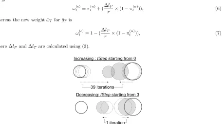
and impoversihment. One way to achieve this is by starting the computation at timetStep=0 and gradually

increasing thetStepby 0.1 as illustrated in the top plot of Fig. 1. The iteration is stopped when the total

Algorithm 1Replicate by gravity.

Generate new set of particles{(gt(c), ω

(c)

t ), c= 1, ..., C}whereC=N

1: s¯T =zt

2: likelihood massmT = 1∗scale

3: foreach particle in{(s(tn), π

(n)

t ), n= 1, ..., N} do

4: s¯i P =s

(n)

t

5: update weightπt(n)=p(zt|xt=s

(n)

t )

6: particle massmP =π

(n)

t ∗scale

7: if πt(n)≥thresholdτ ANDc < C then

8: calculateFt,aP, andaT (Section (3.1))

9: isShif ted= 0

10: tStep=k

11: whileNOTisShif tedANDtStep >0do

12: calculate ∆lP and ∆lT using (3)

13: if (∆lP+∆lT

r )<0.8then

14: isShif ted= TRUE

15: g¯P = (¯sT−s¯iP)×(

∆lP

r ) + ¯s i P

16: ω¯P using (6)

17: g¯T = (¯siP−s¯T)×(∆_rlT) + ¯sT

18: ω¯T using (7)

19: end if

20: tStep=tStep−0.1

21: end while

22: assigngt(c),ω

(c)

t ,g

(c+1)

t andω

(c+1)

t , with ¯gP, ¯ωP, ¯gT and ¯ωT, respectively

23: c=c+ 2

24: else

25: Use Algorithm 2

26: end if

27: end for

is time consuming and requires 39 iterations to move two particles with weigths 0.4 and 1 placed at positions

x=20 andx=180, respectively to reach a total displacement of greater than 80% with the finaltStep=3.8.

A better way to achieve this is to start the computation at timetStep=k, and gradually decreasingtStep

by 0.1 until the total displacement is less than 80% as illustrated in the bottom plot of Fig. 1. This time

decreasing iteration requires only 1 iteration withtStepstarting at 3.0 and is thus preferred. Note that the

final locations of the new particles are not the same for both ways. This sub-optimised solution is similar to

the work in [10, 11] where the new particles are generated closer but not too close to the local mode. This

maintains and improves the original Bayesian distribution of the weighted particles. The new weight ¯ωP for ¯

gP is

ω(tc)=π

(n)

t + ( ∆lP

r ×(1−π

(n)

t )), (6)

whereas the new weight ¯ωT for ¯gT is

ωt(c)= 1−( ∆lT

r ×(1−π

(n)

t )), (7)

where ∆lP and ∆lT are calculated using (3).

Figure 1: Two modes of attracting particles (denoted by bold circles): (top) time increasing iteration; and (bottom) time

decreasing iteration. Shaded circles are the final locations of the replicated particles.

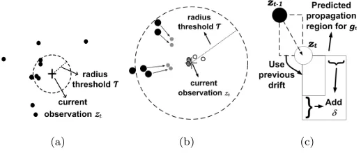
Fig. 2(a) is an example of PF propagation using 10 particles. The particles that fall within the threshold

τ from the current observationztare evaluated using Algorithm 1. The rest of the particles are evaluated using Algorithm 2. We present a quantitative experiment in Section 6.1 to show what threshold value τ

gives GOPF its best performance. Fig. 2(b) is the optimised particles distribution using Algorithm 1 of

GOPF. The four borderless grey circles are the new particles replicated based on where the four particles

(black circles) should move. The four bordered grey circles near the current observationzt are other new particles replicated based on where the virtual particle (atzt) should move. The white bordered circles are the particles propagated by Algorithm 2. Algorithm 1 only replicates the nearby particles. The remaining

(a) (b) (c)

Figure 2: (a) Selecting particles to be replicated; (b) The optimised particles distribution using Algorithm 1 of GOPF; and (c)

Predicted propagation region based on drift (Algorithm 2 of GOPF).

Algorithm 2Propagate within predicted drift region.

1: if (∆ ˙D=zt−zt₋1)<0 then

2: Lˆ= ∆ ˙D−δ

3: Uˆ = 0

4: else

5: Lˆ= 0

6: Uˆ = ∆ ˙D+δ

7: end if

8: fori=c toC do

9: gt(i)=zt+ ˜r mod ( ˆU−Lˆ+ 1) + ˆL

10: update weightωt(i)=p(zt|xt=g( i)

t )

11: end for

Algorithm 2 summarises the propagation procedure based on the PD region. Fig. 2(c) illustrates the

region of possible propagation based on current observation and the PD (indicated by dashed line rectangle),

wherezt₋1andztare respectively the locations of the previous and current observations. The PD region is determined by taking the difference ∆ ˙D={∆ ˙dx,∆ ˙dy}betweenztandzt₋1in both horizontalxand vertical

y directions. The upper and lower values in both directions, denoted as ˆU = {uˆx,uˆy} and ˆL = {ˆlx,ˆly}, respectively, are set accordingly. Depending on ∆ ˙Ddirection, ˆU or ˆLis added (minus for negative direction)

with a thresholdδwhich are then used as an upper and lower bound when propagatinggt(i)with random value ˜

r(line 9 of Algorithm 2). The initial valuecused in the for loop is the last updated index in Algorithm 1,

where C =N, is the total number of newly generated particles based on GOPF. The weight for gt(i) (at line 10 of Algorithm 2) is updated based on the likelihood function defined in (4). GOPF is summarised

in Algorithm 3 where at any time step, the first half consistingN particles are resampled and propagated

based on the PF framework. During the update stage, new set of particles consisting anotherN particles

are generated either using Algorithm 1 or Algorithm 2. They are then combined producing a total of 2N

particles, and are used to estimate the next state.

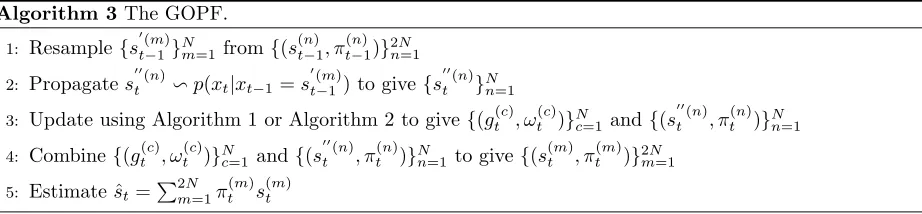
Algorithm 3The GOPF.

1: Resample{s′t(−m1)}

N

m=1 from{(s (n)

t−1, π

(n)

t−1)}

2N n=1

2: Propagates′′t(n)∽p(xt|xt−1=s

′_(m)

t−1) to give{s

′′_(n) t }Nn=1

3: Update using Algorithm 1 or Algorithm 2 to give{(g(tc), ω

(c)

t )}Nc=1 and{(s

′′_(n) t , π

(n)

t )}Nn=1

4: Combine{(gt(c), ω

(c)

t )}Nc=1 and{(s

′′_(n) t , π

(n)

t )}Nn=1 to give{(s (m)

t , π

(m)

t )}2mN=1

5: Estimate ˆst=P

2N m=1π

(m)

t s

(m)

t

4. Hand Features Extraction

The approach taken for hand features extraction in this paper is appropriate for a hand interacting with

an object while facing the camera and with finger bending one at a time. The frontal hand movement is

limited to palm bending within 45◦ _{in X, Y andZ axes.}

One of the distinctive features of a hand is its skin colour. We adapt the implementation of the skin

segmentation for face tracking in [24] for our GOPF based hand tracking framework. With some user

interaction in the first video image frame, the skin colour is extracted. As an analysis of skin colour is not

in within the scope of our current research, a fully automatic initialisation would be considered as a future

work. The input RGB image to the segmentation algorithm is converted into the HSV colour space, and

the hue channel Ih is used to represent the image. Skin segmentation is achieved by matchingIh with a normalised skin colour histogram distributionHskin via back projection. The resulting imageIbp is a single channel image where each pixel inIbp is a probability value of that characterized byHskin, i.e.,

Ibp =p(Ih|Hskin) = p(Ih)

p(Hskin)p(Hskin|Ih). (8)

The largest skin coloured blob is considered to be the hand [12]. A contour is traced onIbp and Douglas-Peucker polygon approximation method [25, 24] is used to reduce the number of redundant contour points

cp.

4.1. Locating Potential Finger Valleys

A convex hull based on Sklansky method [26, 24] is implemented for detecting hand contour, and followed

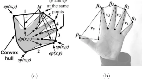
by extracting its convexity defects based on Homma’s method in [18, 24]. Each convexity defect structure

comprises valley/depth point dp(x, y), start point sp(x, y), end point ep(x, y) and depth ld as shown in

Fig. 3(a). There are four significant finger valleys denoted by V = {v0, v1, v2, v3} as shown in Fig. 3(b).

To detect finger valleys of any hand, the four convexity defect structures with the deepest/longest ldare

sequential order in anticlockwise direction. The convexity defects 1, 3, 4 and 5 in Fig. 3(a) are selected to

be the four convexity defects with the deepest/longestld.

(a) (b)

Figure 3: (a) Convex hull and convexity defects of a hand; and (b) labelling fingertips and finger valleys.

4.2. Thumb Localisation and Left/Right Hand Identification

In [17], the labelling of fingertips starts with the localisation of the thumb, where the thumb tip is the

fingertip that is always the farthest away from the average position of all fingertips. Once the thumb has

been found, the rest of the fingertips are indexed according to their distance from the thumb tip. Our

approach is slightly different to [17] by utilising the convexity defects to first locate the thumb valley and

followed by the thumb tip. The subsequent process of labelling the remaining finger valleys and fingertips

is presented in Section 4.3.

Assuming the hand is in outstretched position and is parallel to the image plane, the valley pointdp(x, y)

ofv0, i.e., v0(dp(x, y)), is determined by calculating the maximum accumulated distance adbetween each

valley point with the other three valley points, i.e.,

argmax vc

ad(vc) = m=3

X

i=1

||vc(dp(x, y))−vi(dp(x, y))|| (9)

where vc(dp(x, y)) is the current valley point being analysed, vi(dp(x, y)) is the ith valley point and m is the number of valley points.

Once v0(dp(x, y)) is found, the process then determines if the object is of left or right hand. The

distancedspfrom depth pointv0(dp(x, y)) to start pointv0(sp(x, y)), and the distancedepfrom depth point v0(dp(x, y)) to end pointv0(ep(x, y)) are calculated. Left hand is identified if dep < dsp, otherwise it is a right hand. The thumb tipf t0(x, y) is assigned the end pointep(x, y) or the start pointsp(x, y) depending

on whether it is right hand or left hand, respectively.

4.3. Labelling Finger Valleys and Fingertips

Assumingv0 is found at indexkin ¯V, the remaining valleysviinV wherei={1,2,3}are labelled using

vi= ¯v((k+i) mod 4). (10)

The fingertipsF T ={f ti(x, y), i= 0, ...,4}as shown in Fig. 3(b) are labelled as follows. For left hand, the fingertips are labelled using:

• f t0(x, y) =v0(ep(x, y))

• f t1(x, y) =v1(sp(x, y))

• f t2(x, y) =midpoint(v1(ep(x, y)),v2(sp(x, y)))

• f t3(x, y) =midpoint(v2(ep(x, y)),v3(sp(x, y)))

• f t4(x, y) =midpoint(v3(ep(x, y)),v0(sp(x, y))).

For right hand, the fingertips are labelled using:

• f t0(x, y) =v0(sp(x, y))

• f t1(x, y) =v1(ep(x, y))

• f t2(x, y) =midpoint(v2(ep(x, y)),v1(sp(x, y)))

• f t3(x, y) =midpoint(v4(ep(x, y)),v2(sp(x, y)))

• f t4(x, y) =midpoint(v0(ep(x, y)),v3(sp(x, y))).

During tracking, a new fingertip measurement must be within a certain radius thresholdϕ(determined

experimentally to be 20 pixels for image size 320x240, as larger threshold value will represent a distance

too large for a finger to move to) from the previous measurement, otherwise it is considered missing and

the corresponding valley structurevi will use the previously measuredviprev. For tracking, all non-missing

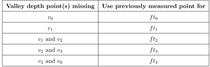
fingertips fromF T are assigned to F T M ={f tMi(x, y), i= 0, ...,4}indicating the measured locations of fingertips. For missing fingertips, the measurement process is presented in Section 4.6. Table 1 shows the

fingertips that use their previously measured point when any or both valley depth points are missing during

the current measurement.

Table 1: Measuring fingertips with missing valley depth point(s).

Valley depth point(s) missing Use previously measured point for

v0 f t0

v1 f t1

v1 andv2 f t2

v2 andv3 f t3

4.4. Determining Finger Pivots

We adapt the method in [27] to determine finger pivots P V = {pvi(x, y), i = 0, ...,4}. A simpler representation is used for the pivots locations, where all finger pivots coincide with the pivot lines as shown

in Fig. 4(a), whereas in [27], three finger pivotspv0(x, y),pv2(x, y) andpv3(x, y) do not. Fig. 4(a) also shows

that only two middle points can be recovered, namely middle (mid23(x, y)) and ring (mid12(x, y)), i.e.,

• mid12(x, y) =midpoint(v1(dp(x, y)),v2(dp(x, y))),

• mid23(x, y) =midpoint(v2(dp(x, y)),v3(dp(x, y))).

(a) (b)

Figure 4: (a) Locations of finger pivots; (b) Finger likelihood region (FLR) enclosed by finger boundaries defined by the left

and right points of a fingertip and a finger valley.

The feature points, i.e., middle point between two depth point valleys, fingertips, and known pivot points,

are used to estimate the pivots of all fingers. Unless otherwise specified, the pivot points are given by

q∗_{= (a−b)×l+a, (11)}

where aand b are feature points, and the distance between two feature points (a−b) is scaled by a ratio

l. By considering the geometry of hand features, the different values ofl are set based on the percentage

difference fromatob. The process is applied to bothxandyelements of each point. Pivot pointspv1(x, y),

pv2(x, y),pv3(x, y) andpv4(x, y) are calculated by making the following substitutions in (11):

• q∗_=pv

2, a=mid12, b=f t2, l= 0.2,

• q∗_=pv

3, a=mid23, b=f t3, l= 0.2,

• q∗_=pv

1, a=pv2, b=pv3, l= 1.2,

• q∗_=pv

4, a=pv3, b=pv2, l= 1.2.

pv1(x, y),pv2(x, y),pv3(x, y) andpv4(x, y) are connected to form the main pivot line (see Fig. 4(a)).

To findpv0(x, y), a temporary location is calculated similarly using (11), whereq∗=temp, a=pv4, b=

pv3, l= 2.8. This is followed by a rotation of 90◦ perpendicular to the main pivot line, i.e.,



   

pv0(x)

pv0(y)

1     

=hR3

i     

temp(x)

temp(y)

1      (12) where

R3=



   

cosβ −sinβ pv4(x)(1−cosβ) +pv4(y) sinβ

sinβ cosβ pv4(y)(1−cosβ)−pv4(x) sinβ

0 0 1

     , (13)

β =−π

2 for left hand andβ =

π

2 for right hand. pv0 and pv4 are connected to form the thumb pivot line

(see Fig. 4(a)). When allP V andF T are extracted, all finger axesF A={f ai(x, y), i= 0, ...,4}are formed by connecting every fingertipf ti with its corresponding finger pivotpvi, denoted by f ai.

4.5. Finger Likelihood Region

Each finger likelihood region (FLR) (see Fig. 4(b)) is used to determine whether a contour pointcpi(x, y) on hand contourQhand is within a specific FLR. FLR is determined by partitioning each finger using the positions of fingertips and finger pivots. Every pivot point has its corresponding left and right points

respectively denoted bypvLi(x, y) and pvRi(x, y), wherei= 0, ...,4 correspond to the numbering of finger pivots. pvR1(x, y),pvL4(x, y) andpvL0(x, y) are calculated by making the following substitutions in (11):

• q∗_=pvR

1, a=pv1, b=pv2, l= 0.6,

• q∗_{=pvL4, a=pv4, b=pv3, l= 0.6,}

• q∗_{=pvL0, a=pv0, b=pv4, l= 0.4.}

ForpvR0(x, y), (11) is slightly modified toq∗= (a−b)×l+b, whereq∗=pvR0, a=pv4, b=pv0, l= 0.4.

pvL1(x, y),pvL2(x, y) andpvL3(x, y) are the midpoints between two adjacent finger pivots, i.e.,

pvL1= (pv1+pv2)/2, pvL2= (pv2+pv3)/2, pvL3= (pv3+pv4)/2. (14)

Since finger pivots pv1(x, y), pv2(x, y), pv3(x, y) and pv4(x, y) are close to each other and the palm

is assumed to be a rigid object, some of pvLi(x, y) share the same point with its adjacent pvRi+1(x, y),

i.e., pvR2 = pvL1, pvR3 =pvL2 and pvR4 = pvL3. Similar to finger pivots, every fingertip has its own

left and right points denoted respectively by f tLi(x, y) and f tRi(x, y), where i = 0, ...,4 correspond to the numbering of fingertips. Denote a new temporary fingertip as f tT empi(x, y) as the location for every fingertip. f tT empi(x, y) is located 13% (based on every finger axis length) away from its corresponding fingertip location along the finger axis, i.e.,

The 13% extension is to create sufficient search space for contour points along fingertips so that the

bound-aries at the fingertips do not lie exactly on top of every fingertip. The line connecting f ti(x, y) and f tT empi(x, y) is extended 120% more to create a new line connectingf tT empi(x, y) andtempi(x, y), i.e.,

tempi= (f tT empi−f ti)×1.2 +f tT empi. (16)

tempi(x, y) is rotated 90◦ _{to the left to obtainf tLi(x, y) and to the right to obtainf tRi(x, y), i.e.,}



   

f tLi(x) f tLi(y)

1     

=hR3

i     

tempi(x) tempi(y)

1      (17)     

f tRi(x) f tRi(y)

1     

=hR3

i     

tempi(x) tempi(y)

1      , (18)

where β =−π

2, and i= 0, ...,4. Fig. 4(b) shows the FLR for each finger. We define the FLR asF LRi=

{pvLi(x, y), pvRi(x, y), f tLi(x, y), f tRi(x, y)}, comprising four points that define the boundaries, where i= 0, ...,4 corresponds to the finger number.

A separate image IF LR is created with the same size as the input image frameIbp. IF LR is used as a lookup table to determine everycpi should they fall into anyF LRi. IF LRarray is first set to zero. Once an F LRi is determined, every pixel inIF LR which corresponds to a pixel enclosed byF LRi is set to i. This results in every finger region having pixel value that corresponds to the finger number.

4.6. Fingertip Measurement during Finger Bending

Precise fingertip measurement during finger bending is not practical for a real-time application and using

only skin colour segmentation will fail to track the edge of a fingertip while it is bending. We thus propose

Algorithm 4 as an approximate solution to fingertip measurement during finger bending.

In Algorithm 4, all contour points cpm of hand contour Qhand are evaluated, and in each iteration, every two consecutive contour pointscpcur(x, y) and cpnext(x, y) are extracted. Pixel value atcpnext(x, y) inIF LR is stored inval1. For every fingertip inF T, ifval1contains a valuei(indicating thatcpnext(x, y) is

withinF LRi), and iff tiuses its previous values, then the linelncur connectingcpcur(x, y) andcpnext(x, y) is evaluated to determine if it intersects with the corresponding finger axis f ai. The pixel locations in IF LR that correspond to the pixel locations along linelncur are first set to a valuek. Define the following determinants: A= a b c d

, B=

e f g h

, C=

Algorithm 4Finding fingertips during bending.

1: foreachcpm(x, y) inQhand,m= 1, ..., N do 2: cpcur(x, y) =cpm(x, y)

3: cpnext(x, y) =cpm+1(x, y)

4: lncur=fromcpcur(x, y) tocpnext(x, y)

5: val1=get pixel value fromIF LR at point cpnext(x, y)

6: foreachf ti(x, y) inF T,i= 0, ...,4 do

7: if val1=i ANDf ti(x, y) uses previous valuethen

8: setIF LR tok for all pixels alonglncur

9: ip(x, y) = intersection point oflncur andf ai axis

10: if ip(x, y) withinIF LR framethen

11: val2=get pixel value fromIF LR at point ip(x, y)

12: if val2=k then

13: f tMi(x, y) =ip(x, y)

14: end if

15: end if

16: end if

17: end for

18: end for

D= b 1 d 1

, E=

e 1 g 1

, F=

f 1 h 1 , (20)

where cpcur(x, y) = (a, b), cpnext(x, y) = (c, d), f ti(x, y) = (e, f) and pvi(x, y) = (g, h). The intersection pointip(x, y) between the linelncur and finger axisf ai is

ip(x) =

A C B E C D E F

, ip(y) =

A D B F C D E F (21)

The resultingip(x, y) is for the infinitely long lines, i.e., an intersection point can occur beyond the two

line segments. To determine whetherip(x, y) lies on both line segments, a pixel value inIF LRcorresponding to the positionip(x, y) is extracted and stored temporarily in val2. If val2 is the same as k then ip(x, y)

v0(dp(x, y)),v1(dp(x, y)) andv2(dp(x, y)) are measured.

Figure 5: A hand contour showing the index finger while bending. Fingertipf t4 uses the previously measured value. The top

left circle shows an enlarged version of the edge of the bending finger. lncuris the line connecting two consecutive contour

points, andip(x, y) is the intersection point betweenlncurand the finger axis.

5. Hand Tracking Framework

GOPF is applied after the features extraction process to maintain the stability of the tracking of

finger-tips, especially during noisy measurements or occlusion. A validation gate mechanism is used in Algorithm 5

as a means to detect outliers in the measurement off ti such as missing or misplaced features during mea-surements. Validation gate radiusvgatei (initially set to 20 pixels for image size 320x240) for fingertip i is introduced to check if the distance between newly measuredf tit and the previously measured f tit−1 is

less than vgatei. If f tit is accepted, vgatei is reduced as well as ensure that the reduction does not fall

below the validation gate thresholdτvgate (normally set to 20 pixels). On the other hand, if the distance is greater than vgatei, the validation gate vgatei is increased. The increment of vgatei is checked to ensure that it is no larger than 4 times the validation gate thresholdτvgate. At this point, the newly measuredf ti is invalidated and considered to be an outlier since it is too far from the previous measurement. Therefore,

f ti has to use the current state estimation ˆst. When this occurs, the fingertipiis in occlusion or currently experiencing noisy measurement. The increase in the size ofvgatei will be used in the next measurement in new frame in order to enlarge the search space.

After f ti is updated in Algorithm 5, and if fingertip i is in occlusion, f ti is again iteratively checked against the extracted contour to search for the closest contour peak tof ti that is withinτvgate radius. If a peak is found,f ti is updated to that peak.

Algorithm 5Outliers detection with validation gate.

1: foreachf ti,i= 0, ...,4 do

2: if distance(f tit,f tit−1)< vgatei then 3: vgatei=vgatei−(τvgate/2)

4: if vgatei< τvgate then

5: vgatei=τvgate

6: end if

7: else

8: vgatei=vgatei+ (τvgate/2)

9: if vgatei>(τvgate×4)then

10: vgatei=τvgate×4

11: f ti= ˆst

12: end if

13: end if

14: end for

6. Experimental Results

A synthetic experiment is used to compare the performance of GOPF with PF [7]. A simulation of a

nonlinear movement is used to compare GOPF with variants of PF. The robustness of the proposed hand

tracking algorithm is validated using real hand video sequences, where comparison is also carried out with

state-of-the-art CAMSGPF. Occlusion handling performance is also performed on both synthetic and real

video sequences. All experiments are performed on Intel Core 2 Duo 2 GHz processor with 4GB RAM.

OpenCV 2.1 is used as the programming environment.

6.1. Synthetic Experiment

A simple mouse tracker program is developed for which PF [7] and GOPF are applied to track the

mouse movement as shown in Fig. 6. This experiment is performed in order to find the best parameter

settings for GOPF to achieve robust performance. Fig. 7 shows the performance of PF and GOPF with

different thresholdτ values. It shows that GOPF outperforms PF for all values of τ, andτ = 0.2 gives its

best performance where the average error decreases as the number of particles increases. As the number

of particles increases,τ <0.2 results in degraded performance because more particles are replicated using

Algorithm 1 instead of Algorithm 2. Forτ >0.2, the opposite happens. Largerτ values tend to give better

results, but most replicated particles would be too concentrated at the true posterior, which results in low

Figure 6: Mouse movement used in a synthetic experiment.

Figure 7: Performance of PF and GOPF in tracking mouse movement.

We simulate a random mouse movement (comprising 3,717 frames) where the mouse moves from different

directions and going through a virtual square-shaped occlusion located at the centre of the screen as shown in

Fig. 8. There are no measurements whenever the mouse enters the virtual occlusion. We compare PF using

100 particles against GOPF using 20 particles and thresholdτ= 0.2 on occlusions handling. The high peaks

of the results in Fig. 9 indicates that the mouse is entering the virtual occlusion, and that GOPF outperforms

PF during occlusion. The average error in the first 200 frames just before the first occlusion is 3.62 for PF

and 3.03 for GOPF. Even without the occlusion, GOPF with 20 particles still performs better than PF with

100 particles. Fig. 10 shows the tracking estimation results of PF and GOPF between frames 200 and 300

which corresponds to the first peak in Fig. 9. Immediately after entering the occlusion boundary, PF tends

to get stuck at the last known measurement and slowly drifts downwards but still within the vicinity of the

last known measurement as shown in Fig. 10. GOPF however produces more reasonable tracking prediction

using the last known mouse movement drift. It tends to follow the actual mouse movement even though

there are no measurements during occlusion.

Figure 8: Random mouse movement passing through a virtual square-shaped occlusion.

Figure 9: Tracking errors of PF and GOPF during occlusion.

6.2. Simulation

We compare the performance of GOPF with several variants of particle filters namely extended Kalman

filter (EKF) [28], sampling importance resampling PF (SIRPF) [29], auxiliary PF (APF) [30], and regularised

PF (RPF) [31] using the nonlinear movement of an object whose position is represented by [32]

xt= xt−1

2 +

25xt−1

1 +x2

t₋1

+ 8 cos(1.2(t−1)) +wt, (22)

and

yt= x2

t

20+jt, (23)

wherewtandjtare zero mean Gaussian random variables with variances 10 and 1, respectively, representing a severely nonlinear model. The works in [33, 29, 34, 21] use this movement to evaluate the performance

of various particle filter algorithms. Root Mean Squared Error (RMSE) is used as a quantitative measure

of performance. All variants including GOPF use 100 particles. The results in Table 2 are obtained by

averaging the RMSE errors over 100 runs for each variant. We also added 5%, 10%, 15% and 20% zero

Figure 10: Tracking estimation of PF and GOPF between frames 200 and 300 of the random mouse movement.

presence of different noise levels. Although the performance of GOPF degrades with increasing noise level,

Table 2 shows that GOPF consistently and significantly outperforms all other algorithms at all noise levels.

Consistent with the results demonstrated in [21], APF always shows slightly better performance compared

to SIRPF and RPF, whereas SIRPF and RPF always show comparable performance.

Table 2: RMSE performance of variants of particle filter with different noise levels.

Algorithm 0% 5% 10% 15% 20%

EKF 23.88 30.48 46.48 53.15 62.91

SIRPF 5.58 6.23 7.84 8.59 9.74

APF 5.19 6.04 7.16 7.96 9.05

RPF 5.24 6.37 7.89 8.51 9.69

GOPF 4.49 5.24 6.41 7.19 8.42

6.3. Qualitative Analysis

A real video sequence is used to evaluate the proposed hand tracking framework. The sequence comprises

416 frames of 320x240 colour images running at 30 fps of a hand with the palm parallel to the camera image

plane, and captured using Logitech Quickcam 3000. In this sequence, each finger is bending one at a time

starting with the thumb, followed by index, middle, ring and pinky. The first frame shows the hand with all

fingers in stretched position. A small region of skin colour is manually sampled in the first frame to be used

for skin colour segmentation in the subsequent frames. In the first frame, all finger valleys and fingertips

are identified and labelled using the methods in Section 4.1 to Section 4.5. GOPF using 20 particles and

τ = 0.2 is then applied to track every fingertip in the subsequent frames where it is observed that the

tracking operates at the video rate of 30 fps. Fig. 11 shows some qualitative comparisons of hand tracking

using PF [7] and GOPF. Note that the measurement noise causes the measured fingertips to not lie exactly

at the actual positions. The result using GOPF optimises the tracking towards the true posterior with an

Figure 11: First, second and third row are results from frame 129, 221, and 295, respectively. Left column shows example of

hand tracking using PF with 10 particles, middle column are the corresponding results using GOPF with 20 particles, and

right column shows the corresponding results using PF with 1000 particles. White lines denote the predicted positions and

black lines denote the measured positions. Black circles denote the fingers entering the missing mode and the fingertips are

measured using Algorithm 4.

GOPF is also applied to a sequence in [35]. This sequence comprises 600 frames of 228x284 colour images

of hand bending one finger at a time starting from thumb, followed by index, middle, ring and pinky. Our

hand tracking framework is able to track the whole sequence reliably. Fig. 12(a) shows the sequence at frame

326 where the middle finger is bending with all other fingers successfully tracked. Pinky and ring fingers

appear closer towards each other, merging them to a single contour as shown in Fig. 12(b). However, the

tracking framework is still able to track the two fingers separately.

(a) (b)

Figure 12: (a) Frame 326 of the sequence in [35]. (b) The corresponding hand contour for frame 326. The white dashed circle

6.4. Hand Tracking: PF vs. GOPF

To validate the performance of GOPF quantitatively, the same sequence as in Fig. 11 is used to compare

its tracking results against the ground truth. Since it is difficult to obtain ground truth data for real hand

video sequence, a common approach [16][35] to a quantitative evaluation of hand tracking is to use a manually

annotated ground truth. Every fingertip is manually annotated and stored inF T GT ={f tGTi(x, y), i= 0, ...,4}. Fig. 13 shows the average error of tracking the five fingers, defined as

average error =

4

X

i=0

|f tMi−f tGTi|

5 . (24)

wheref tMi are the positions of fingertips determined by PF [7] or GOPF. Clearly, GOPF with fewer than 50 particles far outperforms PF with more than 1000 particles. According to [20, 16], and as shown by our

experiment, increasing the number of particles does not improve the accuracy significantly.

Figure 13: Performance of PF and GOPF in hand tracking.

6.5. GOPF vs. PF and CAMSGPF

GOPF is further compared with PF [7] and CAMSGPF [11]. Using the state vector of every propagated

particles as the measurement vector, CAMSGPF works by re-applying or re-measuring the current image

using the simplified CamShift, moving every particle close to the true local mode. GOPF attracts nearby

propagated particles towards the true local mode using gravitational concept without involving any

re-measurement. As reported in [11], CAMSGPF using only 10 particles shows comparable performance with

PF using 100 particles. We applied CAMSGPF using 10 particles to track a moving hand in a real video

sequence comprising 80 frames as shown in Fig. 14. The hand is moving from the right to the left of the

frame.

The result in Fig. 15 shows the comparable performance of CAMSGPF using 10 particles and PF using

100 particles. It is clear that PF using only 10 particles performs worst. Some significant spikes can be seen

Figure 14: A frame in the video sequence of a hand moving from right to left.

considerable stability. The same pattern can be seen in the tracking result on the hockey sequence in [11],

where CAMSGPF shows some fluctuations at frames 400 to 450 of the sequence. This shows some slightly

poor performance of CAMSGPF using 10 particles than with PF using 100 particles in term of stability.

Fig. 15 shows GOPF with 10 particles is more stable compared to PF using 100 particles. The average

errors in tracking are 5.2 for CAMSGPF using 10 particles, 13.6 for PF using 10 particles, 4.2 for PF using

100 particles, and 4.1 using GOPF. The poor performance in the average error of CAMSGPF is partly due

to its optimisation process that might converge into false local mode.

Figure 15: Performance of GOPF vs. CAMSGPF and PF in tracking video sequence in Fig. 14.

6.6. Hand tracking under different hand movements

The performance of the hand tracking framework in tracking a long video sequence comprising 924

frames of different hand movements is also evaluated. The sequence starts with the hand moving closer and

slowly moving farther away from the camera, and then back to its original position. This type of movement

has the effect of scaling the object larger or smaller. The hand then moves up and down which shows the

object translation from one position to another. All these movements maintain the palm to be parallel

to the camera. The movements right after this point do not maintain the palm parallel to the camera.

The wrist is bent forward and backward, moving the fingertips closer and farther away from the camera,

respectively. The movement is stopped when the wrist has turned roughly 45◦ _{during forward or backward}

from the camera, respectively. Again, the movement is limited to twisting the hand at roughly 45◦ _during

forward or backward movement. Fig. 16 shows the framework is able to track all movements successfully

and reliably, where the predicted positions of fingers (denoted by white lines) coincide with the measured

positions (denoted by black lines).

(a) (b) (c) (d)

(e) (f) (g) (h)

Figure 16: Performance of GOPF in tracking different type of hand movements in a single video sequence: (a) moving closer

and (b) moving farther from camera; (c) moving up and (d) down; (e) bend hand forward; (f) bend hand backward; (g) twist

hand with thumb forward; and (h) twist hand with thumb backward. White lines denote the predicted positions and black

lines denote the measured positions.

6.7. Hand tracking in challenging environment

The performance of GOPF with 20 particles to track hand movement in cluttered background is

evalu-ated. The video sequence used in this experiment comprises 710 frames of size 320x240, where a hand enters

the scene performing various movements that involve scaling, rotation and translation. The result in Fig. 17

shows successful tracking of the hand throughout the video sequence.

GOPF is also evaluated with a more challenging environment in a video sequence containing 585 frames of

size 320x240, where the background as well as the foreground contain skin coloured objects. The foreground

contains left and right hands where each hand moves closer towards the camera interchangeably. In this

sequence, GOPF is used to track the left hand. Fig. 18 shows the results of the hand tracking. Initially,

only the left hand is present and is tracked as shown in frame 24. In frame 158, the right hand enters the

scene and as the right hand moves closer towards the camera, its contour becomes the largest skin coloured

blob to be detected. However, the hand tracking framework is able to maintain lock on the left hand. In

frames 162 and 432, the left hand contour are distorted by a skin coloured background. However, the hand

tracking framework successfully maintains correct tracking of the hand in these frames. The results on this

sequence demonstrate the ability of GOPF to successfully track the hand under significant illumination

changes especially when the hand moves closer or away from the camera, i.e., even though deformed hand

Figure 17: Hand tracking in cluttered environment. First to fourth rows are results from frame 48, 484, 496 and 598, respectively.

Left column shows the frames and right column shows the frames with the results (i.e., black lines superimposed onto the frames)

of the hand tracking using GOPF with 20 particles.

contours are extracted.

6.8. Occlusion handling

To evaluate the performance of GOPF with 20 particles for occlusion handling in real image video, a

sequence comprising 319 frames of left hand moving randomly and being occluded twice by an object is

used. Fig. 19 shows the results where frame 101 shows the tracking before the occlusion. The circle on

each fingertips shows the validation gate. At frame 101, the validation gates are at their minimum radius

of 20 pixels. As the occlusion occurs in frame 107, all fingers cannot be measured and the validation gates

for all fingertips increase. As the occlusion disapears in frame 119, fingertips pinky, ring, and middle have

fully recaptured new measurements and their validation gates return to minimum radius. Index fingertip

is still minimizing the validation gate, while thumb fingertip has just recovered new measurement. When

the occlusion completely dissapears at frame 121, almost all fingertips’ validation gates have returned to

Figure 18: Hand tracking in the presence of other skin-colour objects. First row to fourth row are results from frame 24, 158,

162 and 432, respectively. The left column shows the actual frame, the middle column shows the detected contour of the hand,

and the right column shows the results (i.e., black lines superimposed onto the frames) of the hand tracking using GOPF with

20 particles.

7. Conclusions

In this paper, we propose a novel tracking algorithm GOPF by incorporating PF and the replication of

new particles based on gravitational attraction which improves the sampling efficiency as well as significantly

reducing the required number of particles compared to PF. The hand features extraction algorithm which

utilises the convex hull and the convexity defects of the hand shape robustly detects and labels each finger,

as well as identifying if they are of the left or right hand. In terms of accuracy, the GOPF based tracking

outperforms the PF based tracking including various well known variants of PF such as EKF, SIRPF,

APF and RPF. GOPF also outperforms the state-of-the-art CAMSGPF algorithm in terms of stability.

Integration and animation with an OpenGL hand model is the focus of future work where the use of stereo

imaging technique will be incorporated to increase the accuracy of 3D pose estimation. The proposed GOPF

based hand tracking framework has several limitations, and are subject to improvement in future works. The

hand features extraction method may fail in the event the palm twists more than 45◦_{. Complete occlusion for}

a longer period of time might cause the tracker to fail. Fewer parameters usage is preferable in hand features

extraction to avoid missing many parts of the parameters during extraction. Lastly, threshold parameters

(a) (b) (c) (d)

Figure 19: Performance of GOPF in occlusion handling. The results from left to right are from frames 101, 107, 119, and 121

of the sequence. The circle on each fingertip shows the validation gate. The validation gate increases when occlusion occurs,

and decreases when new measurement is found.

are set in pixels unit and mostly work for image size of 320x240. Although threshold parameters can be

adjusted for different image sizes, it is not intended to be used for this framework as it may degrade the

speed (when using large image size) or the accuracy (when using small image size) of the tracking framework.

Acknowledgments

The authors would like to thank the Ministry of Higher Education Malaysia and International Islamic

University Malaysia for providing the funds for this research.

References

[1] H. Francke, J. Ruiz-del Solar, R. Verschae, Real-time hand gesture detection and recognition using boosted classifiers and

active learning, in: D. Mery, L. Rueda (Eds.), Advances in Image and Video Technology, Vol. 4872 of Lecture Notes in

Computer Science, Springer Berlin / Heidelberg, 2007, pp. 533–547.

[2] X. Chai, Y. Fang, K. Wang, Robust hand gesture analysis and application in gallery browsing, in: Proceedins of IEEE

International Conference on Multimedia and Expo, Vol. 1 - 3, 2009, pp. 938 –941.

[3] R. Y. Wang, J. Popovi´c, Real-time hand-tracking with a color glove, ACM Transactions on Graphics 28 (2009) 63:1–63:8.

[4] D. Lee, Y. J. Lee, Framework for vision-based sensory games using motion estimation and collision responses, IEEE

Transactions on Consumer Electronics 56 (3) (2010) 1356 –1363.

[5] A. Chan, H. V. Leong, S. H. Kong, Real-time tracking of hand gestures for interactive game design, in: Proceedings of

IEEE International Symposium on Industrial Electronics, 2009, pp. 98 –103.

[6] A. Erol, G. Bebis, M. Nicolescu, R. D. Boyle, X. Twombly, Vision-based hand pose estimation: A review, Journal on

Computer Vision and Image Understanding 108 (1-2) (2007) 52 – 73.

[7] M. Isard, A. Blake, Condensation - conditional density propagation for visual tracking, Internationa Journal on Computer

Vision 29 (1998) 5–28.

[8] M. Isard, A. Blake, Icondensation: Unifying low-level and high-level tracking in a stochastic framework, in: Proceedings

of the 5th European Conference on Computer Vision, Vol. I, 1998, pp. 893–908.

[9] M. Bray, E. Koller-Meier, L. Van Gool, Smart particle filtering for high-dimensional tracking, Journal on Computer Vision

and Image Understerstanding 106 (2007) 116–129.

[10] C. Shan, T. Tan, Y. Wei, Real-time hand tracking using a mean shift embedded particle filter, Pattern Recognition 40

[11] Z. Wang, X. Yang, Y. Xu, S. Yu, Camshift guided particle filter for visual tracking, Pattern Recognition Letters 30 (2009)

407–413.

[12] I. Oikonomidis, N. Kyriazis, A. Argyros, Efficient model-based 3d tracking of hand articulations using kinect, in:

Pro-ceedings of the 22nd British Machine Vision Conference, BMVA, University of Dundee, UK, Aug. 29-Sep. 1, 2011, pp.

101.1–101.11.

[13] W.-Y. Chang, C.-S. Chen, Y.-D. Jian, Visual tracking in high-dimensional state space by appearance-guided particle

filtering, IEEE Transactions on Image Processing 17 (7) (2008) 1154 –1167.

[14] J. Romero, H. Kjellstrom, D. Kragic, Monocular real-time 3d articulated hand pose estimation, in: Proceedings of the 9th

IEEE-RAS International Conference on Humanoid Robots, 2009, pp. 87 –92.

[15] Y. Wu, J. Lin, T. Huang, Analyzing and capturing articulated hand motion in image sequences, IEEE Transactions on

Pattern Analysis and Machine Intelligence 27 (12) (2005) 1910 –1922.

[16] N. Stefanov, A. Galata, R. Hubbold, A real-time hand tracker using variable-length markov models of behaviour, Computer

Vision Image Understing 108 (2007) 98–115.

[17] Y. Shen, S. K. Ong, A. Y. C. Nee, Vision-based hand interaction in augmented reality environment, International Journal

on Human-Computer Interaction.

[18] T. E. Homma K, An image processing method for feature extraction of space-occupying lesions, Journal of Nuclear

Medicine 26 (1985) 1472–1477.

[19] J. Deutscher, I. Reid, Articulated body motion capture by stochastic search, International Journal on Computer Vision

61 (2005) 185–205.

[20] M.-F. Ho, C.-Y. Tseng, C.-C. Lien, C.-L. Huang, A multi-view vision-based hand motion capturing system, Pattern

Recognition 44 (2011) 443–453.

[21] M. Arulampalam, S. Maskell, N. Gordon, T. Clapp, A tutorial on particle filters for online nonlinear non-gaussian bayesian

tracking, IEEE Transactions on Signal Processing 50 (2) (2002) 174 –188. doi:10.1109/78.978374.

[22] K. A. R. L. Pearson, The Problem of the Random Walk, Nature 72 (1867) (1905) 342.

[23] I. Cohen, A. Whitman, I. Newton, The Principia Mathematical Principles of Natural Philosophy, University of California

Press, 1999.

[24] G. Bradski, A. Kaehler, Learning OpenCV: Computer Vision with the OpenCV Library, O’Reilly, Cambridge, MA, 2008.

[25] D. H. Douglas, T. K. Peucker, Algorithms for the reduction of the number of points required to represent a digitized line

or its caricature, Cartographica: The International Journal for Geographic Information and Geovisualisation 10 (2) (1973)

112–122.

[26] J. Sklansky, Finding the convex hull of a simple polygon, Pattern Recognition Letters 1 (2) (1982) 79 – 83.

[27] E. Yoruk, E. Konukoglu, B. Sankur, J. Darbon, Shape-based hand recognition, IEEE Transactions on Image Processing

15 (7) (2006) 1803 –1815. doi:10.1109/TIP.2006.873439.

[28] H. W. Sorenson, Kalman filtering: theory and application., IEEE, 1985.

[29] N. Gordon, D. Salmond, A. Smith, Novel approach to nonlinear/non-gaussian bayesian state estimation, IEEE Proceedings

F, Radar and Signal Processing 140 (2) (1993) 107–113.

[30] M. K. Pitt, N. Shephard, Filtering via Simulation: Auxiliary Particle Filters, Journal of the American Statistical

Associ-ation 94 (446) (1999) 590–599.

[31] C. Musso, N. Oudjane, F. Legland, Improving regularized particle filters, in: A. Doucet, N. de Freitas, N. Gordon (Eds.),

Sequential Monte Carlo Methods in Practice. New York, springer-verlag Edition, Statistics for Engineering and Information

Science, 2001, pp. 247–271.

[32] G. Kitagawa, Non-gaussian state-space modelling of non-stationary time series (with discussion), Journal of the American

Statistical Association 82 (1987) 1032–1063.

[33] N. G. P. Bradley P. Carlin, D. S. Stoffer, A Monte Carlo Approach to Nonnormal and Nonlinear State-Space Modeling,

Journal of the American Statistical Association 87 (418) (1992) 493–500.

[34] G. Kitagawa, Monte carlo filter and smoother for non-gaussian non-linear state space models, Journal of Computer

Graphics and Statistics 5 (1) (1996) 1–25.

[35] M. de La Gorce, D. Fleet, N. Paragios, Model-based 3d hand pose estimation from monocular video, IEEE Transactions