Development of solid state NMR techniques for the characterisation of pharmaceutical compounds

(1)

University of Warwick institutional repository: http://go.warwick.ac.uk/wrap

A Thesis Submitted for the Degree of PhD at the University of Warwick

http://go.warwick.ac.uk/wrap/51660

This thesis is made available online and is protected by original copyright.

Please scroll down to view the document itself.

(2)

www.warwick.ac.uk

AUTHOR: Andrew Stephen Tatton DEGREE: Ph.D.

TITLE:Development of Solid-State NMR techniques for the characterisation of pharmaceutical compounds

DATE OF DEPOSIT: . . . .

I agree that this thesis shall be available in accordance with the regulations governing the University of Warwick theses.

I agree that the summary of this thesis may be submitted for publication.

Iagreethat the thesis may be photocopied (single copies for study purposes only).

Theses with no restriction on photocopying will also be made available to the British Library for microfilming. The British Library may supply copies to individuals or libraries. subject to a statement from them that the copy is supplied for non-publishing purposes. All copies supplied by the British Library will carry the following statement:

“Attention is drawn to the fact that the copyright of this thesis rests with its author. This copy of the thesis has been supplied on the condition that anyone who consults it is understood to recognise that its copyright rests with its author and that no quotation from the thesis and no information derived from it may be published without the author’s written consent.”

AUTHOR’S SIGNATURE: . . . .

USER’S DECLARATION

1. I undertake not to quote or make use of any information from this thesis without making acknowledgement to the author.

2. I further undertake to allow no-one else to use this thesis while it is in my care.

DATE SIGNATURE ADDRESS

. . . .

(3)

Development of Solid-State NMR techniques for

the characterisation of pharmaceutical compounds

by

Andrew Stephen Tatton

Thesis

Submitted to the University of Warwick

for the degree of

Doctor of Philosophy

Department of Physics

(4)

LIST OF TABLES

3.1 Selection of ∆p = +1 coherence order change by phase cycling. . . 54 3.2 Full phase cycle for a DQ correlation experiment. . . 54

4.1 Effective13C-1H couplings and T2’ times obtained from fitting the

ex-perimental data for L-alanine in Fig. 4.4 for a 32µs eDUMBO-122 cycle. 80

4.2 Effective13C-1H couplings and T2’ times obtained from fitting the

ex-perimental data for L-alanine in Fig. 4.4 for a 24µs eDUMBO-122 cycle. 80

4.3 13C fitting parameters for spin-echo curves . . . 83

5.1 15_{N GIPAW calculated and experimental isotropic chemical shift values}

for cimetidine. . . 107

6.1 A comparison of15N and14N experimental and GIPAW calculated shifts

for dG(C3)2. . . 130

6.2 NH distances up to 3 ˚A in dG(C3)2, extracted from the geometry

opti-mised (CASTEP) crystal structure. One-bond correlations are denoted

in bold and intermolecular correlations shown in italic. . . 131

for cimetidine . . . 139

7.2 NH distances up to 3 ˚A in cimetidine form A, extracted from the

geom-etry optimised (CASTEP) crystal structure. One-bond correlations are

(9)

7.3 A comparison for cimetidine between experimental1H isotropic chemical

shifts and isotropic chemical shifts calculated using the GIPAW method

for the full crystal structure and an isolated molecule. . . 142

7.4 NH distances within 3 ˚A proximity taken from the geometry optimised

(CASTEP) crystal structures of nicotinamide (top) and nicotinamide

palmitic-acid (bottom). One-bond correlations are denoted in bold, and

intermolecular correlations are denoted in italic. . . 144

for nicotinamide (top) and nicotinamide palmitic-acid (bottom). . . 146

7.6 A comparison of 15N and 14N experimental isotropic shifts for PVP,

(10)

LIST OF FIGURES

1.1 Schematics of a pharmaceutical salt, cocrystal and amorphous solid

dis-persion. . . 7

2.1 Representation of energy levels for an isolated spin-½ nucleus when the

degeneracy of the energy levels is lifted . . . 13

2.2 Vector representation of a pulse in the rotating frame . . . 24

2.3 Euler angles defined in Cartesian coordinates . . . 27

2.4 Energy level diagram for two-coupled spin-½nuclei when no dipolar

cou-pling is present, heteronuclear dipolar coucou-pling only is considered, and

all dipolar couplings are considered . . . 30

2.5 Simulated NMR lineshape for a heteronuclear dipolar coupling between

two spin-½ nuclei . . . 32

2.6 Simulated powder pattern showing a CSA lineshape, acquired usingη= 0.5 . . . 35

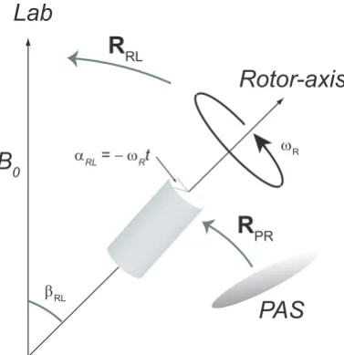
2.7 Illustration of a rotor aligned atβRL relative to theB0 . . . 37

2.8 Perturbation to the Zeeman energy levels for a spin-1 nucleus when

considering the first-order and second-order perturbation due to the

quadrupolar interaction . . . 41

3.1 Simulated 1D NMR lineshapes showing absorptive and dispersive

line-shapes . . . 48

3.2 Simple 2D NMR pulse sequence . . . 49

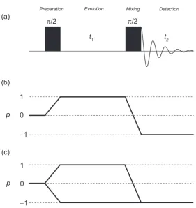
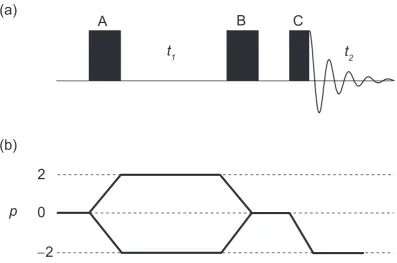
3.3 Pulse sequence and coherence pathway for a DQ correlation experiment 55

(11)

3.5 Schematic of the Lee-Goldburg condition and FSLG sequence . . . 58

3.6 Phase modulation curve for an eDUMBO-122 complete cycle . . . 60

3.7 Ramped CPMAS pulse sequence . . . 62

3.8 NMR pulse sequence for a general heteronuclear spin-echo experiment . 64

3.9 Calculated heteronuclear spin-echo modulation curves for a range of CHn

systems . . . 66

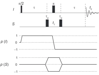
3.10 NMR pulse sequence for a 2D HMQC experiment . . . 68

4.1 13C-1H heteronuclear spin-echo pulse sequence . . . 75

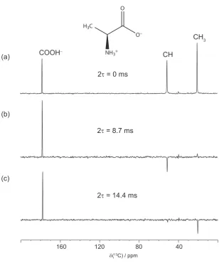
4.2 1J13C-1H edited spectra of L-alanine, recorded for a range of τ periods . 77

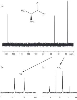
4.3 13C one-pulse solution-state spectrum of L-alanine . . . 78

4.4 13C spin-echo modulation curves of the CH and CH3 group in L-alanine

acquired using different homonuclearrf nutation frequencies and decou-pling cycle times . . . 79

4.5 13C spin-echo curves acquired using a 24 µs homonuclear decoupling cycle time at spinning frequencies of 20.833 kHz and 25 kHz . . . 81

4.6 Comparison between13C homonuclear spin-echo curve and13C

heteronu-clear spin-echo curve, using heteronuheteronu-clear or homonuheteronu-clear decoupling

duringτ. . . 82 4.7 13C-1H spin-echo simulated modulation curves recorded with and

with-out heteronuclear dipolar coupling under static conditions . . . 85

4.8 Comparison between 2-spin 13_C-1_{H spin-echo curves and corresponding}

spectra obtained applying FSLG and eDUMBO-122 during τ periods,

where different heteronuclear interactions are present. . . 87

4.9 Spin-echo curves presented in Fig. 4.8, an additional1H CSA interaction

is included. . . 89

4.10 2-spin 13C-1H spin-echo curves recorded using FSLG decoupling during

τ periods for numerous single crystallite orientations. . . 91 4.11 Comparison between 13C-1H spin-echo modulation curves for a 2-spin

CH system and 8-spin CH7 system recorded using different FSLG and

(12)

4.12 Simulated 13C-1H spin-echo curves obtained for a CH group

employ-ing eDUMBO-122 decoupling during τ periods, comparing the effect of

different cycle times and corresponding suitablerf nutation frequencies 94 4.13 Comparison between simulated 13_C-1_{H spin-echo curves obtained for a}

CH group and a CH3 group . . . 95

5.1 Rotor-synchronised and non rotor-synchronised1J15N-1Hmodulation curves

of singularly labelled L-histidine.HCl.H2O . . . 104

5.2 1J15N-1Hspectral editing spectra obtained for dipeptideβ-AspAla recorded

at variousτ values . . . 106 5.3 1J15N-1H spectral editing spectra obtained for cimetidine recorded over a

rangeτ values . . . 108 5.4 1_J

15N-1Hspectral editing spectra obtained for tenoxicam form III recorded

over a range ofτ values . . . 109 5.5 1J15N-1H spectral editing spectra obtained for pazopanib recorded using

variousτ increments . . . 111

6.1 14N-1H HMQC pulse sequence . . . 116

6.2 14N-1H HMQC spectrum obtained for the dipeptide β-AspAla at an MAS frequency of 60 kHz. . . 119

6.3 14N-1H HMQC spectrum obtained for the dipeptide β-AspAla at MAS frequencies of 30 kHz, 45 kHz, and 60 kHz. . . 121

6.4 1H rows taken through the NH and NH+₃ sites from 2D HMQC spectra

obtained for the dipeptideβ-AspAla, for a range of τRCPL times. . . 122

6.5 NH dipolar build-up curves obtained for the NH and NH+₃ site from

HMQC spectra obtained for dipeptide β-AspAla, for a range of τRCPL

times. . . 125

6.6 14N-1H J-HMQC spectrum obtained for dipeptide β-AspAla . . . 127 6.7 Skeletal structure for a deoxyguanosine derivative . . . 128

6.8 14N-1H HMQC spectrum obtained for dG(C3)2 at different dipolar

re-coupling durations . . . 129

(13)

7.2 Comparison between X-ray single crystal structure relative to geometry

optimised structure of cimetidine . . . 140

7.3 14N-1H HMQC spectra of cimetidine recorded at different recoupling

durations . . . 141

7.4 Skeletal structure of the nicotinamide palmitic-acid cocrystal . . . 144

7.5 2D14N-1H HMQC experiments of nicotinamide and nicotinamide

palmitic-acid . . . 145

7.6 15N CPMAS spectra of nicotinamide and nicotinamide palmitic-acid . . 147

7.7 2D14N-1H HMQC spectra recorded for PVP, acetaminophen and a

PVP-acetaminophen dispersion . . . 149

7.8 1H one-pulse spectra of PVP (not-dried), PVP (dried), acetaminophen

and a 50% w/w PVP-acetaminophen dispersion . . . 150

7.9 15_{N CPMAS spectra of (a) PVP, (b) acetaminophen and (c) 50 % w/w}

(14)

ACKNOWLEDGMENTS

Firstly, I wish to thank my supervisor, Professor Steven Brown, for all his help, support

and encouragement over the past few years, including giving me the opportunity to work

on interesting projects, allowing me to travel to a variety of destinations in the name of

science and for always being willing to read through my work. I would also like to thank

everybody at GSK for their help, particularly Tran Pham for taking a real interest in

my work and for helping me see how solid-state NMR fits into the pharmaceutical

industry, also thanks to Fred Vogt, Simon Watson and Andy Edwards for their help at

various stages throughout my project and time at GSK. I would also like to thank all

members of the Warwick group, particularly Dinu Iuga for his help with the 14N-1H experiments, and Jon Bradley for all his help and discussions throughout the thesis,

particularly with the computational work. Also, I would like to thank Paul Hodgkinson

for all his help in the homonuclear decoupling project. Financial support from EPSRC

and GSK is gratefully acknowledged.

Outside of NMR, I would like to thank all the friends I have met at Warwick

over all the last 8 years, as well as those from outside of Warwick, and back home.

Finally, I would like to give a special thanks to all my family for their constant love

(15)

DECLARATIONS

All work performed in this thesis is original research carried out by this author, unless

otherwise stated, in the Department of Physics at the University of Warwick, under the

supervision of Professor Steven P. Brown between October 2008 and June 2012. An

exception is experimental results in chapter 5, which were carried out by the author

in the structural characterisation group at GlaxoSmithKline, Stevenage, UK, in the

periods June 2010 to July 2010 and May 2011 to June 2011.

Some of the results presented have been published. Specifically, results from chapter 4:

A. S. Tatton, I. Frantsuzov, S. P. Brown and P. Hodgkinson. Unexpected effects

of third-order cross-terms in heteronuclear spin systems under simultaneous

radio-frequency irradiation and magic-angle spinning NMR. J. Chem. Phys., 136:084503, 2012. [1]

Results in chapter 5 and chapter 7:

A. S. Tatton, T. N. Pham, F. G. Vogt, D. Iuga, A. J. Edwards and S. P. Brown. Probing

intermolecular interactions and nitrogen protonation in pharmaceuticals by novel 15

N-edited and 2D14N1H solid-state NMR. CrystEngComm, 14:2654-2659, 2012. [2]

Results in chapter 6:

A. L. Webber, S. Masiero, S. Pieraccini, J. C. Burley, A. S. Tatton, D. Iuga, T. N.

Pham, G. P. Spada, and S. P. Brown. Identifying Guanosine Self Assembly at Natural

(16)

(17)

ABSTRACT

Structural characterisation in the solid state is an important step in understand-ing the physical and chemical properties of a material. In pharmaceuticals, an active pharmaceutical ingredient (API) may be medicinally favourable, but have undesirable physical properties, such as poor solubility, that potentially limit further development. Solid delivery forms, such as pharmaceutical salts, cocrystals and solid amorphous dispersions, potentially offer improvements in physical properties, whilst maintaining favourable medicinal characteristics. Solid-state NMR is an extremely sensitive probe of the local atomic environment and intermolecular interactions, for example hydrogen bonding, and is therefore well suited to studies of pharmaceuticals.

Solid-state NMR techniques applied to solid delivery forms are presented as an alternative to more established structural characterisation methods. The effect of homonuclear decoupling upon heteronuclear couplings is investigated using a combina-tion of experimental and density-matrix simulacombina-tion results acquired from a13_C-1_H

spin-echo pulse sequence, modulated by scalar couplings. It is found that third-order cross terms under MAS and homonuclear decoupling contribute to strong dephasing effects in the NMR signal. Density-matrix simulations allow access to parameters currently unattainable in experiment, and demonstrate that higher homonuclear decoupling rf

nutation frequencies reduce the magnitude of third-order cross terms. 15N-1H spin-echo experiments were applied to pharmaceutically relevant samples to differentiate between the number of directly attached protons. Using this method, proton transfer in an acid-base reaction is proven in pharmaceutical salts.

(18)

ABBREVIATIONS

API Active Pharmaceutical Ingredient

BABA BAck-to-BAck

CP Cross Polarisation

CRAMPS Combined Rotation And Multiple Pulse Spectroscopy

CSA Chemical Shift Anisotropy

DFT Density Functional Theory

DSC Differential Scanning Calorimetry

DQ Double-Quantum

DUMBO Decoupling Using Mind Boggling Optimisation

EFG Electric Field Gradient

FID Free Induction Decay

FSLG Frequency-Switched Lee-Goldburg

FT Fourier Transform

FWHMH Full Width at Half Maximum Height

GIPAW Gauge-Including Projector Augmented Waves

HETCOR Heteronuclear Correlation

HMQC Heteronuclear Multiple Quantum Coherence

INEPT Insensitive Nuclei Enhanced by Polarisation Transfer

MAS Magic Angle Spinning

NMR Nuclear Magnetic Resonance

PAS Principal Axis System

PMLG Phase-Modulated Lee Goldburg

ppm Parts Per Million

(19)

REPT-HSQC Recoupled Polarisation Transfer Heteronuclear Single-Quantum Cor-relation

rf Radio-Frequency

SCXRD Single Crystal X-ray Diffraction

SDG Solvent Drop Grinding

S/N Signal-to-Noise

SPINAL Small Phase INcremental ALternation

SQ Single-Quantum

TPPI Time Proportional Phase Increment

TPPM Two Pulse Phase Modulated

(20)

CHAPTER

ONE

INTRODUCTION

1.1 Solid-State NMR development

Since the independent observations of the magnetic resonance phenomena by Purcell [4]

and Bloch, [5] nuclear magnetic resonance (NMR) has rapidly progressed to become

a key characterisation tool in chemistry laboratories throughout the world. NMR is a

site-specific tool which is sensitive to subtle changes in chemical environments.

Char-acterisation in the solid state is often more appropriate than liquid state analysis. For

example, details concerning molecular packing configurations, such as hydrogen

bond-ing and polymorphism are specific to the solid phase. In solution, molecular tumblbond-ing

usually occurs on a faster timescale to that of the NMR interactions, which averages

out broadening effects, resulting in narrow lineshapes and the simple extraction of

chemical shift parameters. Consequently, the majority of NMR experiments are

usu-ally performed in the solution state. In the solid state, molecular tumbling does not

usually occur, therefore anisotropic effects with an orientational dependence are not

averaged by motional effects, leading to broad, featureless lineshapes that hinder

ex-traction of chemical shift information. Solid-state NMR lineshapes are not lacking in

information, rather the overload of structural information hinders analysis, contrasting

to the solution state where analysis is simplified by narrow lineshapes.

A significant breakthrough in solid-state NMR was the independent invention

of magic angle spinning (MAS) in the 1950’s by Andrew [6,7] and Lowe. [8] The

(21)

whose root is arctan√2 ≈ 54.7◦, known as the magic angle. If samples in the solid

state are rotated at the magic angle relative to the external magnetic field, B0, then

a majority of anisotropic interactions average out over a complete rotor period, as if

subject to molecular tumbling in the solution state. Improvements in probe

technol-ogy has seen the introduction of ever smaller rotor diameters: currently the smallest

diameter conventional probe commercially available is 1.0 mm, capable of achieving

spinning frequencies approaching 80 kHz. [9] MAS is able to resolve sufficiently

nar-row lines for lower-γ nuclei, such as 13C and 15N, where the dominant interaction is the chemical shift anisotropy, however MAS does not completely average strong,

non-commuting homonuclear (1H-1H,19F-19F) dipolar couplings. This is problematic when

analysing organic materials consisting of dense proton environments, as the

homonu-clear dipolar coupling is dependent upon the square of the gyromagnetic ratio and the

internuclear distance between the coupled nuclei to the inverse cubed power. 1_{H has}

the highest gyromagnetic ratio of NMR active nuclei (except for3H) and in organic

ma-terials close range proton-proton proximities are typically short (approximately 2-3 ˚A),

therefore applying MAS alone does not sufficiently average strong dipolar couplings,

which are tens of kHz in magnitude, and therefore severely hinder resolution in

or-ganic materials, such as pharmaceuticals. In order to average strong, non-commuting

homonuclear dipolar couplings, homonuclear dipolar decoupling sequences have been

developed, which involve the application of carefully choreographed radio-frequency

(rf) nutation frequency to a sample.

The first demonstration of using rf irradiation to average homonuclear dipolar couplings and consequently obtain narrower lineshapes was the Lee-Goldburg

tech-nique, applied to CaF2 to obtain narrow 19F lineshapes. [10] This consists of

off-resonance continuousrf irradiation, which rotates the spin-component of the magneti-sation at an effective field aligned at the magic-angle relative toB0. Further decoupling

sequences were introduced, such as WaHuHa (WHH), [11, 12] which is composed of a

series of on-resonance rf pulses of differing phase and evolution periods. The first decoupling schemes were designed for use in static cases. Whilst adequately

averag-ing homonuclear dipolar couplaverag-ings, other anisotropic interactions, such as the chemical

shift anisotropy (CSA), are not averaged by such decoupling pulse sequences. In

(22)

however the combination of both methods, known as Combined Rotation and Multiple

Pulse Sequences (CRAMPS) [13–15] can potentially result in significant improvements

in spectral resolution.

Frequency Switched Goldburg (FSLG) [16, 17] and Phase Modulated

Lee-Goldburg (PMLG) [18] are improvements of the Lee-Lee-Goldburg sequence, [10] and are

examples of homonuclear decoupling sequences applicable in the CRAMPS approach.

FSLG applies a series of off-resonance, effective 2π pulses with alternating, opposite signed frequencies. The Decoupling Using Mind Boggling Optimisation (DUMBO)

[19, 20] family of decoupling sequences, including an experimentally optimised version,

e-DUMBO-122, [21] involve the application of constant amplitude rf irradiation with

rapid switching of the phase, and are also commonly applied CRAMPS methods. Both

FSLG and eDUMBO-122 are applied extensively throughout this thesis, and are

ex-plained in greater detail in chapter 3. The successful use of ever more complicating

decoupling schemes owes much to the advent of more sophisticated hardware capable

of delivering consistent, rapid phase shifts and high rf nutation frequencies.

CRAMPS is an important experimental consideration in a heteronuclear

spin-echo experiment, which has been presented previously as a method for identifying

different CHngroups. [22, 23] Spin-echo sequences are of great importance in a range of

magnetic resonance applications and were first proposed by Hahn in 1950, [24] and

fur-ther developed by Carr and Purcell in 1954. [25] By refocusing the evolution due to

in-homogeneous broadening, coherence lifetimes, as described byT2’ dephasing times, are

extended, consequently reducing the corresponding (spin-echo) linewidths. A typical

1_J

13C-1H coupling is approximately 100 Hz, whereas the heteronuclear dipolar coupling

between a chemically bonded CH pair is approximately 20 kHz. Therefore, averaging

of strong heteronuclear and homonuclear dipolar couplings, in addition to refocusing of

inhomogeneous broadening effects, is usually necessary to achieve sufficient resolution

to observe a CH or NH Jsplitting. Different through-bond multiplicities yield specific splitting patterns, that can be resolved provided that the acquisition of narrow

spin-echo lineshapes is achieved; in this way, the presence of through-bond coupling(s) can

be proved.

The implementation of spin-echo pulse sequence elements modulated by

(23)

Two-dimensional heteronuclear correlation experiments, such as J-HMQC, [27], J -HSQC, [28] refocused INADEQUATE, [29–31] and the refocused INEPT sequence,

[32, 33] all employ a spin-echo during the pulse sequence, and exploit magnetisation

transfer via through-bond couplings. 2D experiments consist of two evolution

peri-ods, therefore allowing for interactions that are not directly observable in an NMR

experiment to be indirectly probed. In addition to 2D experiments where coherence

transfer occurs by isotropic J couplings, correlation via anisotropic couplings, such as the dipolar coupling, are an important tool in solid-state NMR.

Whilst anisotropic interactions hinder spectral resolution, they also contain

valu-able structural information, therefore the total removal of all anisotropic interactions is

not always desirable. For example, the dipolar interaction, which is inversely dependent

on the cube of the distance between coupled nuclei is a valuable source of information on

internuclear distances. Therefore, re-introducing the dipolar coupling, which is removed

by MAS, in a controlled manner is a powerful method for identifying intramolecular and

intermolecular proximities. Recoupling of heteronuclear or homonuclear dipolar

cou-plings is possible using different recoupling schemes. Heteronuclear dipolar recoupling

schemes include rotary resonance recoupling (R3), [34] and Rotational-Echo Double

Resonance (REDOR), [35] whereas schemes such as Dipolar Recovery at the Magic

Angle (DRAMA), [36] POST-C7, [37] and R-based sequences [38] are used to recouple

homonuclear dipolar couplings.

The dipolar coupling interaction is directly utilised in the cross polarisation (CP)

experiment. The sensitivity of a lower-γ nucleus, such as 13C and 15N, is enhanced by coherence transfer from an abundant nucleus, typically protons, through the dipolar

couplings by achieving the Hartmann-Hahn matching condition. [39] Additionally, as

1_{H nuclei typically have shorter} _T

1 times relative to 13C or 15N, CP can reduce the

experimental time compared to direct acquisition. Initially, CP experiments were

ac-quired under static conditions, [40,41] however CP is typically now applied under MAS

conditions. [42]13C CPMAS is considered as a workhorse solid-state NMR experiment

of organic materials, e.g., for pharmaceutical applications, [43] owing to its relatively

simple set-up, acceptable experimental times and the rich information content available.

Insight into internuclear proximities can be gained from two-dimensional

(24)

2D experiments which utilise cross-polarisation, such as 13C-1H HETCOR

experi-ments. [44–46] Alternatively, the dipolar coupling can be reintroduced for indirect

observation using recoupling schemes; for example1H double-quantum correlation

ex-periments. [47] Heteronuclear Multiple-Quantum Coherence (HMQC) experiments have

been demonstrated utilising either through-bond couplings, [27, 48, 49] or via the

re-coupling of heteronuclear dipolar re-couplings. [50] HMQC experiments can be used to

achieve correlation between two spin-½nuclei, such as13C-1H, or correlation between a

spin-½ nucleus and a quadrupolar nucleus, such as14N. [51]

Computational techniques are a very useful complement to experimental data.

The development of Hamiltonian propagator governed density-matrix simulation

pro-grams such as Simpson [52] or SPINEVOLUTION [53] are advantageous as they allow

the user to investigate the viability of new experiments or complement existing

experi-mental results. Furthermore, they allow access to experiexperi-mental conditions not currently

possible due to hardware limitations, and removal of specific interactions that are not

of direct interest can aid understanding.

First-principles calculations utilising DFT (density functional theory) has rapidly

progressed in solid-state NMR. The CASTEP platform [54] uses planewave

pseudopo-tentials [55] to reconstruct the electron density throughout a material. Crystalline

materials are particularly suited to CASTEP calculations, as they exploit periodicity

in the crystal lattice. DFT calculations are ideally suited to optimising light-element

positions determined by single crystal diffraction. GIPAW (gauge included

projec-tor augmented waves) [56–59] calculations using the CASTEP platform yield isotropic

chemical shifts and EFG (electric field gradient) parameters to assist in the

assign-ment of experiassign-mental data. GIPAW calculations of NMR parameters in a diverse range

of systems has been demonstrated, [3, 60–63] including application to pharmaceutical

molecules. [64–67]

1.2 Characterisation of pharmaceutical solids

Solid-state NMR is an increasingly applied methodology in pharmaceutical analysis.

[43, 68–70] Demonstrated applications include identifying different polymorphic forms,

(25)

the relative amorphous and crystalline content of pharmaceuticals, [75, 76] studies of

dynamics within a pharmaceutical molecule, [77] and analysis of drug products. [78, 79]

1.2.1 Pharmaceutical formulations

Pharmaceutically interesting compounds with medicinally favourable properties will

not always have desirable physical properties such as bio-availability, solubility and

chemical stability. Numerous solid delivery forms are utilised to improve physical

prop-erties of an active pharmaceutical ingredient (API), [80] including but not limited to

pharmaceutical salts, [81] cocrystals, [82–85] and solid amorphous dispersions. [86, 87]

It is important, for both patent and regulatory reasons, that suitable screening of

phar-maceutical solid forms are available, as small changes in molecular structure can have

a significant impact upon the performance of a drug.

The most prominent multi-component delivery forms in the pharmaceutical

in-dustry are pharmaceutical salts. However, these are reliant upon the API being

suf-ficiently ionisable. Despite the high proportion of pharmaceutical salts, the accessible

design space of salt formations is considered to be restrictive owing to the relatively

low number of non-toxic pharmaceutical acid or base formers available.

Cocrystals have recently received attention as an alternative to pharmaceutical

salts. A cocrystal is typically, although not universally, defined as two or more neutral

components in the solid phase, which are typically bound by covalent interactions, such

as hydrogen bonding. [88] An amorphous solid-dispersion with a hydrophilic polymeric

carrier maintains the advantageous solubility properties associated with the amorphous

state, whilst also improving the thermodynamical stability relative to a free amorphous

phase, which is thermodynamically unstable relative to the crystalline phase. Typically,

intermolecular bonding between individual cocrystal constituents and between an

amor-phous API and corresponding hydrophilic carrier is via hydrogen bonding. Solid-state

NMR has been shown to be an ideal characterisation tool for cocrystals [89–91] and

amorphous dispersions. [92]

Cocrystal discovery utilises the solvent drop grinding synthesis route, discovery

in this manner does not always allow for straightforward growth of a single crystal

nec-essary for characterisation using single crystal X-ray diffraction (SCXRD). To date, full

(26)

charac-API

−/+

+/

−

_+/

−

API

Neutral neutral

co-former Neutral

neutral

co-former hydrophiliccarrier

API

amorphous

API

amorphous

hydrophilic carrier

Pharmaceutical

salt

Pharmaceutical

cocrystal

Pharmaceutical

solid amorphous

dispersion

a

b

c

API

−/+

Figure 1.1: Schematics representation of (a) pharmaceutical salt, (b) pharmaceutical cocrystal and (c) amorphous solid dispersion. This figure is based around Fig. 1 in ref. [84].

terisation techniques. For amorphous materials, traditional structural characterisation

methods, such as single crystal X-ray diffraction (SCXRD), are not suitable due to

a lack of long-range order. Solid-state NMR is applicable to materials that are

non-crystalline. Differential scanning calorimetry (DSC) techniques are currently the most

prominent screening technique for solid amorphous dispersions, however interpretation

of more complex systems has been shown to be challenging, particularly if glass

tran-sition temperature values (Tg) of separate components are similar (within 10◦C). [93] Solid-state NMR is applicable to more complex systems, and furthermore, is able to

accurately pinpoint the positions of lighter elements, such as 1H, which are often not

easily determined using diffraction techniques. Schematic representations of various

solid delivery forms which are of interest in the pharmaceutical industry are shown in

Fig. 1.1.

1.2.2 Hydrogen bonding

A hydrogen bond is a non-covalent interaction between a proton donor X-H, and an

electronegative proton acceptor Y, commonly the Y nucleus is nitrogen, oxygen or

fluorine. Hydrogen bonds are of particular interest as the interaction is strong enough

to hold together molecules. By defining a hydrogen bond as X-H...Y, where X is directly

bonded to the proton and Y is more electronegative than H, the strongest hydrogen

bonding occurs when XY is at the shortest separation, as X-H and H...Y distances

(27)

molecule or as an intermolecular interaction.

Solid-state NMR has been demonstrated as a powerful probe of hydrogen

bond-ing configurations. [95] The1H isotropic chemical shift is most deshielded (highest ppm)

when the hydrogen bonding is strongest. [15, 96, 97] Additionally, changes in hydrogen

bonding geometry can be identified from changes in extracted quadrupolar parameters,

this has been demonstrated for numerous quadrupolar nuclei, including 14N,35Cl and

17_{O. [60, 98, 99] Recently, it has been shown that GIPAW calculations can assist in}

identifying and quantifying specific hydrogen bonding interactions. This is achieved

through comparison of calculated 1H chemical shifts of a full crystal structure relative

to an isolated molecule. The isotropic proton chemical shift of the isolated molecule is

found to be less deshielded relative to the full crystal, dependent upon the strength of

the hydrogen bond interaction. [67, 100–102]

1.2.3 Nitrogen solid-state NMR methods

Nitrogen is present in a majority of pharmaceuticals compounds, and often is directly

involved in acid-base interactions or hydrogen bonding interactions. Both naturally

occurring nitrogen isotopes are NMR active, each possessing different challenges, and

providing different information content. 14N has a natural abundance of 99.6%

com-pared to 0.37% 15N abundance. 14N has a lower gyro-magnetic ratio and is spin-1

compared to spin-½for15N. Nuclei with spin greater than spin-½ possess a quadrupolar

interaction arising from interaction between the nuclear quadrupole moment and the

electric field gradients at the nucleus. This interaction can be of the order of MHz and

results in broad lineshapes that are only partially averaged by MAS, as explained in

more detail in section 2.4.5. However, the quadrupolar coupling, whilst hindering

spec-tral resolution, yields electric field gradient (EFG) parameters which are inaccessible

from spin-½15_{N NMR.}

15_{N is a spin-}_½ _{nucleus and is therefore not complicated by the presence of}

the quadrupolar interaction. As is shown in this thesis, the identification of different

XHn functional groups (where X = 13C or 15N) can be achieved by establishing the

number of through-bond coupling(s) using spectral editing methods. J-based spectral

editing methods, referred to herein as 1J15N-1H editing for15N analysis, achieved using

(28)

of directly attached protons to a spin-½ nucleus. [22] An inspection of signal changes

over a range of τ values allows for the identification of different proton moieties as the magnetisation evolves according to the number of covalent bonds. As discussed, the

most common multi-component delivery method of an API are pharmaceutical salts,

which are composed of an ionised acid-base pair. Nitrogen sites often act as a proton

acceptor during an acid-base reaction, therefore establishing the presence of proton

transfer via the presence of a through-bond N-H coupling is a potentially powerful

method for establishing whether a salt has formed.

Studies of 14N have been limited relative to 15N studies owing to unfavourable

spin-1 properties, despite its much higher natural abundance. Indirect detection of14N

via 1H offers improvement in signal relative to direct 14N detection. This is achieved

herein using 2D14N-1H HMQC experiments, [51] where if the correlation mechanism is

dipolar coupling then qualitative information regarding intra and intermolecular

prox-imities can be extracted. Probing the state of protonation in nitrogen functional groups

and identifying hydrogen bonding configurations is a valuable tool during

pharmaceu-tical development.

1.3 Thesis Outline

This thesis details the development and application of solid-state NMR for

pharma-ceutical characterisation. Solid-state NMR is shown to be a well suited technique for

probing pharmaceutical salts, cocrystals and amorphous solid-dispersions.

Addition-ally, windowless homonuclear dipolar decoupling sequences are investigated using a

combination of experimental and density-matrix simulation results, particularly within

the context of heteronuclear experiments.

Chapter 2 outlines the relevant theory concerning solid-state NMR. The

un-derlying quantum mechanics is presented and Hamiltonian descriptions of key NMR

interactions detailed. Experimental principles that are used within the thesis are

intro-duced in chapter 3. Explanations of phase cycling, NMR lineshapes and 2D experiments

of general relevance to solid-state NMR are detailed, in addition to more specialised

techniques such as homonuclear decoupling and particular pulse sequences used in this

(29)

DFT GIPAW calculations are introduced.

Chapter 4 concerns the effect of homonuclear decoupling upon CH

heteronu-clear couplings, which was established using a combination of experiment and

density-matrix simulations. It is well documented that homonuclear decoupling schemes scale

isotropic interactions, including J couplings, however the important effect upon het-eronuclear dipolar couplings was not previously realised. Experimental hethet-eronuclear

spin-echo modulation curves are presented for L-alanine, acquired using eDUMBO-122

homonuclear decoupling during τ periods, for a range of cycle times and rf irradia-tion frequencies. Further understanding of the effect of homonuclear decoupling upon

heteronuclear dipolar couplings is achieved using simulation results. The capability to

include specific interactions of interest allows the relevance of separate interactions to

be established. Although simulations were initially performed for a single CH spin pair,

the number of spins was increased in order to gauge the effect of introducing additional

close range protons. Using simulations, it was possible to record modulation curves for

single crystals, and investigate the effect of rf nutation frequencies and corresponding decoupling cycle times currently not achievable experimentally.

15_{N spectral editing experiments applied to pharmaceutical molecules are}

demon-strated in chapter 5. As nitrogen sites can be protonated in a pharmaceutical salt,

proving protonation is an important regulatory and patent concern. Spectral editing

techniques which utilise through-bond couplings were applied to tenoxicam Form III

and pazopanib, both of which are in the form of pharmaceutical salts. Furthermore, the

1_J

15N-1H technique was applied to cimetidine, a pharmaceutical molecule. Calculated 15_{N isotropic chemical shifts, obtained using the GIPAW method, were used to assist}

in the 15N spectral assignment.

Chapter 6 begins with an investigation of the effect of changing the MAS

fre-quency for14N-1H HMQC experiments of the dipeptideβ-AspAla. Furthermore, com-parison betweenβ-AspAla spectra acquired using correlation transfer via through-bond or through-space couplings is presented. For spectra acquired using correlation transfer

via through-space couplings, the effect of different recoupling durations upon coherence

transfer for various NH proximities was investigated experimentally, and complemented

using simulation to establish semi-quantitative information regarding NH dipolar

(30)

guano-sine derivative is presented in order to establish that the sequence is applicable to

systems beyond model set up materials. GIPAW calculations using CASTEP assist in

the assignment of isotropic chemical shifts and by calculating14N EFG parameters.

Chapter 7 demonstrates application of the 14_N-1_{H HMQC experiment to}

phar-maceutically relevant materials. Firstly, application to cimetidine is demonstrated,

in conjunction with GIPAW calculation. The viability of 2D 14N-1H HMQC

exper-iments as a possible cocrystal and amorphous dispersion screening technique is then

presented. The example cocrystal investigated is nicotinamide palmitic-acid, whereas a

solid amorphous dispersion of an API (acetaminophen) and a hydrophilic carrier (PVP)

was selected. Of particular interest is the potential to probe intermolecular hydrogen

bonding interactions, which indicate molecular association. Cocrystal results are aided

by GIPAW calculation of isotropic chemical shifts and electric field gradient (EFG)

(31)

CHAPTER

TWO

NMR THEORY

When a nuclear spin is subject to a static external magnetic field, interactions between

the magnetic moment and the external field lift the degeneracy of the energy levels. The

energy of transitions between these levels are specific to each nuclear species, and the

strength of the external field. If the sole insight from NMR was distinguishing between

different nuclear species, then the appeal of NMR as a spectroscopic tool would be

limited. However, subtle shifts to the energy of a transition provide valuable insight

into the surrounding environment of the nucleus. Within this chapter, the spin angular

momentum operators for a single spin are introduced, followed by the density operator

formalism, which is a more suitable description for an ensemble of spins. External

and internal NMR interactions are discussed, and individual Hamiltonians for each

interaction are presented. The theory contained within this chapter is based upon that

presented in refs. [103–105].

2.1 Spin Angular Momentum

Spin angular momentum is an intrinsic property of a nucleus, whose magnitude is

quantised in discrete terms of ¯h, where ¯h is equal to Planck’s constant. A possible 2I

+ 1 energy levels exist, where I is the total spin angular momentum quantum number. In the absence of a magnetic field the energy levels are degenerate, however application

of a static, external magnetic field, B0, lifts the degeneracy of the energy levels. This

is due to an interaction between the magnetic moment and B0. The splitting between

(32)

ω

₀

=

−γ

B

₀

No external Application of magnetic field external magnetic

field

m = +½

m =

−

½

(a)

(b)

Figure 2.1: Representation of energy levels for an isolated spin-½ nucleus when (a) not subject to an external magnetic field, and (b) subject to an external magnetic field, therefore the degeneracy of the energy levels is lifted.

is given by:

ˆ

H =−µˆ·B0 (2.1)

The magnetic moment, µˆ is defined as:

ˆ

µ=γIˆ (2.2)

where γ is the gyromagnetic ratio. For a case where the spin angular momentum is aligned along the direction of the external magnetic field, and convention dictates that

this is taken along the z-axis, referred to as the longitudinal direction, the Zeeman

energy Hamiltonian can be written as:

ˆ

H =−γIˆzB0

=ω0Iˆz (2.3)

where ω0 is the Larmor frequency,

ω0 =−γB0 (2.4)

(33)

to the gyro-magnetic ratio, γ, which is a constant for each nuclear species, and the strength of the external magnetic field, B0. NMR yields information content owing

to this splitting in energy levels, which is quantised and is sensitive to subtle changes

in the local environment of a nucleus, which perturb the Zeeman splitting energy by

small, but measurable quantities. Nuclei which have I = 0 (e.g., 12C) have no energy splitting when subject to an external magnetic field, and are therefore not observable

in an NMR experiment.

A wavefunction completely describes all spatial and spin properties of a system

in quantum mechanical terms, and is denoted herein as |ψi. When an operator, ˆA, which represents a desired physical quantity, acts upon a system it yields a value

detailing that physical property. Repeated experiments will yield an average value,

known as the expectation value, which describe the result of a specific operator acting

upon a defined system, given as:

D ˆ

A

E

=hψ|Aˆ|ψi (2.5)

A general operator, ˆA, can be expressed as a matrix, where the elementArs is given as

hr|Aˆ|si:

A=



 

Aφ1φ1 Aφ1φ2

Aφ2φ1 Aφ2φ2

  =   

hφ1|Aˆ|φ1i hφ1|Aˆ|φ2i

hφ2|Aˆ|φ1i hφ2|Aˆ|φ2i





 (2.6)

Observables relating to the nuclear spin can be extracted through application of the

spin-angular momentum operator. The total magnitude of the spin-angular momentum

squared, is given as:

ˆ

I2 = Î_x2+ Î_y2+ Î_z2 (2.7)

The x, y, and z-components of spin-angular momentum, are expressed in matrix form

as:

ˆ

Ix = 

 

0 1₂

1 2 0   , ˆ

Iy =i 

 

0 −1₂

1 2 0   , ˆ

Iz = 

 

1 2 0

0 −1₂ 



(34)

Using the above matrix notations results in the following commutator relations:

h ˆ

I2,Iˆz i

= 0 (2.9)

h ˆ

Ix,Iˆy i

=iIˆz (2.10)

As only a single component of the spin angular momentum commutes with the total

spin angular momentum, this implies that only a single component of the spin angular

momentum is observable at any single point in time, which by convention is the

z-component. As discussed, the z-component is defined as being aligned parallel to the

external field and is referred to as the longitudinal direction, whereas the x-y plane is

defined as the transverse plane. The individual components of spin angular momentum

do not commute with each other, therefore individual components of spin angular

momentum are not observable at the same point in time. The operators ˆI2 and ˆIz, acting upon |ψi, yield the following eigenvalues:

ˆ

I2 |ψi= ¯hI(I+ 1)|ψi (2.11) ˆ

Iz |ψi= ¯hm|ψi (2.12)

wheremis the z-component of the spin-angular momentum, and can take values of−I,

−I+ 1 ... I−1, +I. Therefore, for a spin-½nucleus there are two possible values ofm, namely +1₂ and −1₂, as seen in Fig. 2.1. These eigenstates are defined as spin-up (α) and spin-down (β) respectively. Therefore, the operator ˆIz, acting upon eigenstates|αi and|βi, yield the following eigenvalues:

ˆ

Iz|αi= + 1

2|αi (2.13)

ˆ

Iz|βi=− 1

2|βi (2.14)

As indicated by the x and y-components of the spin angular momentum not commuting

(35)

in conversion to the other eigenstate:

ˆ

Ix|αi= 1

2|βi (2.15)

ˆ

Ix|βi= 1

2|αi (2.16)

ˆ

Iy|αi= 1

2i|βi (2.17)

ˆ

Iy|βi=− 1

2i|αi (2.18)

An isolated spin-½ nucleus is not required to exist purely in one eigenstate, rather it

can be considered as a superposition of α and β states, written as:

|ψi=cα|αi+cβ|βi (2.19)

The expectation value of an operator, hAˆi (recall equations 2.5 and 2.6), acting upon a spin-½nucleus, can expressed as a matrix multiplication:

hAˆi=

c∗_α c∗_β



 

Aαα Aαβ

Aβα Aββ       cα cβ   

=c∗_αcαAαα+c∗αcβAαβ+c∗βcαAβα+c∗βcβAββ (2.20)

The probability of residing in either state depends on cαor cβ , where|cα|2₊_|_cβ_|2 _{= 1.}

Note, that |ψi and hψ|denote column and row vectors, respectively. Therefore, using equation 2.20, the operator ˆIz, acting upon a spin-½ nucleus, yields the expectation value:

D ˆ

Iz E

=hψ|Iˆz|ψi =1

2(cαc ∗

α−cβc∗β) =1

2|cα|

2₋1

2|cβ|

2

(2.21)

Therefore, the implication of equation 2.21 is that the longitudinal component of spin

angular momentum is dependent upon direct-products (c∗_αcα, c∗_βcβ) of the coefficients

for either state, which corresponds to the on-diagonal matrix elements in equation 2.20.

(36)

are cross-products (c∗_αcβ, c∗βcα) between the coefficients which describe either state,

given as:

hIˆxi= 1 2(cαc

∗

β+cβc∗α) (2.22)

hIˆyi= 1 2i(cαc

∗

β−cβc∗α) (2.23)

2.2 The Density Operator

Although the above description is suitable for an isolated spin 1₂ nucleus, to describe

the NMR experiment for an ensemble of spins, where numerous spins are present, is

necessary. A more complete manner of writing the scalar constants, ci, in equation 2.6

is required. This is achieved by expressing an ensemble of spins as a density operator,

which is defined as:

ˆ

ρ= |ψihψ| (2.24)

Here, ˆρ signifies the density operator. It is important to note that the overbar signifies an average over an ensemble of states. However, the overbar notation will be dropped

from further expressions for convenience. The density operator is a more complete

manner of describing a system of many spins. As for the isolated spin-½ nucleus, an

expectation value can be calculated by applying an operator to a system. The density

operator expressed for an ensemble of isolated spin-½ nuclei, in matrix form (the

so-called density matrix) is expressed as:

|ψihψ|=

   cα cβ   

c∗_α c∗_β

=



 

cαc∗α cαc∗β

cβc∗α cβc∗β 



 (2.25)

The product of the density operator and an operator acting upon a system is:

ρA=



 

cαc∗α cαc∗_β

cβc∗α cβc∗β      

Aαα Aαβ

Aβα Aββ    =   

cαc∗αAαα+cαc∗βAβα cαc∗αAαβ+cαc∗βAββ

cβc∗αAαα+cβc∗βAβα cβc∗αAαβ+cβc∗βAββ 



(37)

Inspection of the matrix reveals that the on-diagonal elements correspond to the

ex-pectation value in equation 2.20. Therefore, the exex-pectation value is determined as the

trace of the matrix.

hAˆi= Tr(ρA) (2.27)

Expressing the coefficients in equation 2.19 as a product of a real coefficient, aα or aβ,

and a phase constant, φα orφβ, allows better understanding of the significance of the on and off-diagonal elements of the density matrix.

|ψi=aαeiφα|αi+aβeiφβ|βi (2.28)

Substitution of equation 2.28 into equation 2.24, yields a density operator to describe

a system of isolated spins as:

ρ= 

 

aα2 aαaβei(φα−φβ)

aαaβei(φβ−φα) aβ2





 (2.29)

If all spins reside in subtly different states, taken over an entire system, the values of

ei(φα−φβ)_{will destructively interfere and average to zero, leaving on-diagonal terms only}

in equation 2.29. This is referred to as a population state. Note, that the retention of

on-diagonal terms only is analogous to longitudinal spin angular momentum.

Now consider an ensemble of spins that reside in the same state, therefore,

av-eraged over the whole system, the value of ei(φα−φβ) _{is non zero. Consequently, the}

off-diagonal terms in equation 2.29 are retained. This is referred to as a phase

coher-ence between states. Importantly, only cohercoher-ence states are observable in an NMR

experiment, therefore the spin system must be manipulated from the population state

at thermal equilibrium into an observable phase coherence (in reality, only single

quan-tum coherences are directly observable in an NMR experiment, though other types of

coherence can be indirectly observed in multi-dimensional experiments). The presence

of off-diagonal components is akin to the transverse components of spin angular

mo-mentum, indicating that observation of a coherence requires magnetisation to be in the

(38)

2.2.1 The time dependence of the density operator

An NMR experiment consists of a combination ofrf pulses and free evolution, therefore the density operator must be considered as a time dependent function. Differentiating

the density operator with respect to time gives:

d ˆρ(t) dt =

d

dt(|ψihψ|)

=

d dt |ψi

hψ|+|ψi

d dthψ|

(2.30)

The time dependent Schr¨odinger equations for|ψi and hψ|are:

d

dt |ψi=−i

ˆ

H|ψi (2.31)

d

dthψ|=ihψ|

ˆ

H (2.32)

Therefore, substitution of the above expressions into equation 2.30 gives:

d

dtρˆ(t) =−i

h ˆ

H,ρˆ(t) i

(2.33)

This is known as the Liouville von-Neumann equation, the solution of which is:

ˆ

ρ(t) = ˆU(t) ˆρ(0) ˆU(t)−1 (2.34)

The propagator is defined as ˆU(t), and describes the Hamiltonian acting betweent=0 and t=t. If the Hamiltonian does not change over this period then the propagator is:

ˆ

U(t) =e−iHtˆ (2.35)

Equations 2.34 and 2.35 imply that in order to calculate the time dependent density

operator, then the initial state of the system must be known, in addition to the

Hamil-tonian(s) present during time period t=0 and t=t. However, different Hamiltonian interactions may be present at different points during an NMR experiment, therefore

it is necessary to express the propagator as a series of Hamiltonians, written as:

ˆ

(39)

Note, that the Hamiltonian interactions are taken in chronological order. Individual

Hamiltonian descriptions for relevant interactions are detailed in sections 2.3 and 2.4.

2.2.2 Hamiltonians

A total Hamiltonian operator can be constructed to describe all relevant interactions

which evolve during an NMR experiment. In the context of an NMR experiment,

Hamiltonians can be classed as either an external or internal interaction. The total

Hamiltonian is then considered as a sum of all relevant Hamiltonian interactions:

ˆ

H = ˆHZ+ ˆHrf+ ˆHσ + ˆHD + ˆHQ+ ˆHJ (2.37)

Here, ˆHZand ˆHrf are external interactions representing the Zeeman interaction and rf pulses, respectively, and ˆHσ + ˆHD + ˆHQ + ˆHJ are internal spin interactions, signifying the chemical shielding, dipolar coupling, quadrupolar interaction andJ cou-pling respectively. A Hamiltonian to describe an operator ˆA is expressed in Cartesian coordinates as:

ˆ

HA= ˆIA˜Sˆ

=

ˆ

Ix Iˆy Iˆz      

Axx Axy Axz

Ayx Ayy Ayz

Azx Azy Azz             ˆ Sx ˆ Sy ˆ Sz       (2.38) ˆ

I represents a spin operator I, ˜A describes the interaction and ˆS can be a further interacting spin operator or an external variable.

2.3 External Interactions

Within this section, external interactions between the nuclear spin system and external

(40)

2.3.1 Thermal Equilibrium State

In a static, homogeneous magnetic field, the Hamiltonian describing the interaction

between the external magnetic field and nuclear spin, ˆI, is given as:

ˆ

HZ=−γIˆzB0=ω0Iˆz (2.39)

Therefore, the density operator can be written, using statistical physics, as:

ρ= e −β¯hω0Iz

T r[e−β¯hω0Iz_] (2.40)

where, β = _k1

βT and kβ is Boltzmann’s constant. In the high temperature (T)

approx-imation, which in reality is any temperature a few fractions of a Kelvin above absolute

zero, it follows that β 1. Furthermore, e−n≈(1−n). Therefore, equation 2.40 can be written as:

ρ≈ 1−β¯hω0Iz

T r[e−β¯hω0Iz_] (2.41)

Using the relationship, Tr[A] + Tr[B] = Tr[A+B], and that Tr[1] = 2N, then equation

2.41 can be written as:

ρeq=const.−

β¯hω0

2N Iz (2.42)

ρeq∝Iz (2.43)

This demonstrates that at thermal equilibrium the density operator is aligned along the

z-axis. It is assumed that an NMR experiment always begins at thermal equilibrium,

corresponding to magnetisation aligned along the z-direction in a population state.

Only coherence states are measurable in an NMR experiment, therefore creation of

coherence states between spins is required to observe an NMR signal.

2.3.2 Application of an rf pulse

As demonstrated, at thermal equilibrium the magnetisation resides in a population state

(41)

field, B1, whose oscillation frequency, ωrf is close to ω0, and is consequently capable

of manipulating the magnetisation. ωrf is applied in the radiofrequency range of the EM spectrum. The oscillating magnetic field, in this case aligned along x-direction, is

written as:

B1(t) = 2B1(cos[ωrft+φ])i (2.44)

=B1[exp(+iωrft) + exp(−iωrft)]i if φ= 0

where ±ωrf are counter rotating frequencies of the oscillating pulse, φ is the phase of the pulse and i is a unit vector aligned along the x-direction. The application of an on or close to on resonance rf pulse tilts the magnetisation away from the z-axis, and results in the bulk magnetisation precessing about the z-axis. Since only +ωrf is sufficiently close toω0for the pulse to have an effect upon the magnetisation, the effect

of the−ωrf term upon the magnetisation can be safely ignored. The Hamiltonian for an rf pulse is therefore simplified as:

ˆ

Hrf = Î.Z.˜Bˆ1 =−γB1[ Îxcos(ωrft+φ) + Îysin(ωrft+φ)] (2.45)

By convention, the NMR frame is considered as the x-y axis precessing about the z-axis

at a frequency of +ωrf, known as the rotating frame. Therefore, the rf Hamiltonian can be treated as time independent. In the rotating frame, the radiofrequency field

appears static, and a pulse is simply seen as the application of a static magnetic field

of magnitude B1. Consequently, equation 2.45 can be expressed as:

ˆ

H_rfrot=−γB1[ ˆIxcos(φ) + ˆIysin(φ)] (2.46) =ω1Iˆx if φ= 0

where ω1 is referred to as the nutation frequency of the rf pulse. As demonstrated

in equation 2.46, when the phase of the rf pulse is zero the pulse is applied along the x-axis. In order to change the axis along which a pulse is applied, then the phase of the

(42)

along the x-axis, is given as:

ˆ

ρ(t) =e−iω1tIˆx_ρ₍₀₎_eiω1tIˆx _(2.47)

If the initial state of the system, which is assumed to consist of spin-½ nuclei only, is

a population state, i.e., ρ(0) = ˆIz, then expansion of equation 2.47 into matrix forms gives: [103]

ˆ

ρ(t) = 1 2



 

cos(ω1t) isin(ω1t)

−isin(ω1t) cos(ω1t)





 (2.48)

The expectation values of Îx, Îy and Îzare calculated by taking the trace of the product of equation 2.48, and the relevant spin operator. The expectation values are therefore

calculated as:

D ˆ

Ix E

=T r[ρIx] = 0 (2.49)

D ˆ

Iy E

=T r[ρIy] =−1

2sin(ω1t) (2.50)

D ˆ

Iz E

=T r[ρIz] = 1

2cos(ω1t) (2.51)

The application of anrf pulse, aligned along the x-direction, rotates the magnetisation about the x-axis by a flip angle, defined asβ, relative to the initial magnetisation state. The flip angle is determined by the strength of ω1, and the time for which the pulse is

applied, and is given as:

β =ω1tp (2.52)

A vector representation of the application of a 90◦ pulse applied about x is shown in

(43)

z

y

x

a

b

(90°)_x

M

Figure 2.2: (a) Vector model of magnetisation residing in a population state, aligned parallel to the z-axis in the rotating frame. (b) After application of a 90◦ pulse about x the magnetisation resides in the x-y plane.

2.3.3 Evolution under an offset

Once a coherence state is created, and therf pulse is switched off, then the magnetisa-tion evolves in the transverse plane under a resonance offset. The resonance offset, Ω,

emerges from considering the magnetisation in the rotating frame. It is defined as the

difference between the Larmor frequency of a nucleus and the rf nutation frequency, i.e., Ω =ω0−ωrf. Switching to a rotating frame corresponds to the experimental mix-ing down of the NMR signal with a wave oscillatmix-ing at ωrf. In this way, the oscillating frequencies of the NMR signals are now of the order of kHz, rather than MHz, and are

more manageable. The Hamiltonian which describes evolution under a resonance offset

is defined as:

ˆ

H = Ω ˆIz (2.53)

Therefore, it follows that the time dependent density operator, for initial transverse

magnetisation ˆIx, under a resonance offset is:

ˆ

ρ(t) = 1 2



 

0 e−iΩt eiΩt 0





(44)

An NMR signal is calculated by taking the trace of the product of ρ(t) and a raising operator, ˆI+ (≡Iˆ†−), given as:

ˆ

I+ = ˆIx+iIˆy =    0 1 0 0    (2.55)

The raising operator describes quadrature detection, where both the real and imaginary

component of the free induction decay (FID), corresponding to detection of two

com-ponents perpendicular to each other, are recorded. Quadrature detection is explained

in more detail in section 3.1.1. A detected NMR signal, under a resonance offset, is

therefore given by:

s(t) = Tr[ ˆI+ρˆ]

= Tr       0 1 0 0      

0 e−iΩt eiΩt 0

      = 1

2(cos(Ωt) +isin(Ωt)) (2.56)

The physical manifestation of equation 2.56 is that the transverse magnetisation, recorded

as both a real and imaginary component (90◦phase difference between the two signals),

rotates in the transverse plane, inducing a current in a coil, which corresponds to the

NMR signal.

2.3.4 Product Operators

Product operators are an alternative formalism to density operator theory. Although

not suitable for explaining an ensemble of spins with numerous strong couplings present,

they are adept at cases where weak couplings only are present. The changes in the bulk

magnetisation, due to application of a pulse about the y-axis, of flip angleβ, in product operator formalism, is: [103]

Ix βy

(45)

Additionally, evolution under a resonance offset can also be described using the product

operator formalism:

Ix

Ωt

−→Ixcos Ωt+Iysin Ωt (2.58)

Product operators are also able to describe evolution between weakly J coupled spins, where spins I and S can be the same, or different, nuclear species. The J coupling is an internal interaction between chemically bonded nuclei, and is described in more

detail in section 2.4.6. If magnetisation is considered to initially reside upon ˆIx, then evolution under aJ coupling is, according to the product operator formalism:

Ix πJISt

−→ IxcosπJISt+ 2IySzsinπJISt (2.59)

The second term on the right hand side of equation 2.59 is a two-spin operator,

cre-ated from the product of two single-spin operators, thus showing how the product

operator formalism is able to describe the time evolution of a coupled system. If the

magnetisation is initially upon the I spin, then magnetisation will evolve in time into a coupled state involving the S spin. Product operators are a useful tool to describe pulse sequences that involve magnetisation transfer via a J coupling. For weak inter-actions, evolution under a J coupling and resonance offset can be treated sequentially using product operators, despite the evolution under the distinct interactions occurring

simultaneously.

2.4 Internal Interactions

The external interactions introduced in section 2.3 describe the interactions between

the nuclear spin system and external variables. Internal interactions describe nuclear

spin interactions within a nuclear spin system. The most convenient Hamiltonian

ex-pression for an internal interaction is its principal axis system (PAS), in which the

interaction matrix is the Hamiltonian expression introduced in equation 2.38 is

(46)

β

α α

γ

Z = Za

Zab_{= Z}abc

Yabc

Ya_{= Y}ab Y

Xabc Xab

Xa X

Figure 2.3: Euler angles defined in Cartesian coordinates

typically coincide. As an example, the dipolar coupling lies along the internuclear

vec-tor between the nuclei, however the chemical shielding frame of reference is determined

by the surrounding electronic environment.

Owing to the dominance of the Zeeman interaction, which is aligned parallel

to B0, it is necessary to rotate all remaining interactions to this frame of reference,

referred to herein as the Laboratory frame. Rotations are characterised by three angular

rotations in the Cartesian coordinate system, defined as α, β and γ, and are known as the Euler angles. Initial rotation takes place under α, which rotates the coordinate system from (X,Y,Z) about Z to (Xa,Ya,Za), followed by rotation under the angle β

about Ya, creating a new coordinate system, (Xab,Yab,Zab), and finally rotation under

γ about Zaboccurs, which rotates the axes to (Xabc,Yabc,Zabc). The change in Cartesian coordinates when rotated by the Euler angles are shown in Fig. 2.3. In order to simplify

the mathematical description of a rotation, Hamiltonians are best expressed in spherical

tensor form, which are specified as:

ˆ

H=

2

X

j=0 +j X

m=−j

Development of solid state NMR techniques for the characterisation of pharmaceutical compounds

University of Warwick institutional repository: http://go.warwick.ac.uk/wrap

A Thesis Submitted for the Degree of PhD at the University of Warwick

http://go.warwick.ac.uk/wrap/51660

This thesis is made available online and is protected by original copyright.

Please scroll down to view the document itself.

Development of Solid-State NMR techniques for

the characterisation of pharmaceutical compounds

Andrew Stephen Tatton

Department of Physics

CONTENTS

LIST OF TABLES

LIST OF FIGURES

ACKNOWLEDGMENTS

DECLARATIONS

ABSTRACT

ABBREVIATIONS

ONE

INTRODUCTION

1.1

Solid-State NMR development

1.2

Characterisation of pharmaceutical solids

charac-API

+/

−

+/

−

API

API

API

API

Pharmaceutical

salt

Pharmaceutical

cocrystal

Pharmaceutical

solid amorphous

dispersion

a

b

c

API

1.3

Thesis Outline

TWO

NMR THEORY

2.1

Spin Angular Momentum

ω

=

−γ

B

m = +½

m =

−

½

(a)

(b)

2.2

The Density Operator

2.3

External Interactions

z

z

y

y

x

x

a

b

M

M

2.4

Internal Interactions

_+/