Developing resource consolidation frameworks for moldable virtual machines in clouds

http://wrap.warwick.ac.uk/

Original citation:

He, Ligang, Zou, Deqing, Zhang, Zhang, Chen, Chao, Jin, Hai and Jarvis, Stephen A..

(2014) Developing resource consolidation frameworks for moldable virtual machines in

clouds. Future Generation Computer Systems, Volume 32 . pp. 69-81.

Permanent WRAP url:

http://wrap.warwick.ac.uk/54735

Copyright and reuse:

The Warwick Research Archive Portal (WRAP) makes this work of researchers of the

University of Warwick available open access under the following conditions. Copyright ©

and all moral rights to the version of the paper presented here belong to the individual

author(s) and/or other copyright owners. To the extent reasonable and practicable the

material made available in WRAP has been checked for eligibility before being made

available.

Copies of full items can be used for personal research or study, educational, or

not-for-profit purposes without prior permission or charge. Provided that the authors, title and

full bibliographic details are credited, a hyperlink and/or URL is given for the original

metadata page and the content is not changed in any way.

Publisher statement:

© 2014 Elsevier, Licensed under the Creative Commons

Attribution-NonCommercial-NoDerivatives 4.0 International

http://creativecommons.org/licenses/by-nc-nd/4.0/

A note on versions:

The version presented here may differ from the published version or, version of record, if

you wish to cite this item you are advised to consult the publisher’s version. Please see

the ‘permanent WRAP url’ above for details on accessing the published version and note

that access may require a subscription.

Developing Resource Consolidation Frameworks for Moldable Virtual Machines in

Clouds

Ligang He1, Deqing Zou2, Zhang Zhang2, Chao Chen1, Hai Jin2, and Stephen A. Jarvis1

1. Department of Computer Science, University of Warwick, Coventry, United Kingdom

2. School of Computer Science and Technology, Huazhong University of Science and Technology, Wuhan, China [email protected], [email protected]

Abstract—This paper considers the scenario where multiple clusters of Virtual Machines (i.e., termed as Virtual Clusters) are hosted in a Cloud system consisting of a cluster of physical nodes. Multiple Virtual Clusters (VCs) cohabit in the physical cluster, with each VC offering a particular type of service for the incoming requests. In this context, VM consolidation, which strives to use a minimal number of nodes to accommodate all VMs in the system, plays an important role in saving resource consumption. Most existing consolidation methods proposed in literature regard VMs as “rigid” during consolidation, i.e., VMs’ resource capacities remain unchanged. In VC environments, QoS is usually delivered by a VC as a single entity. Therefore, there is no reason why VMs’ resource capacity cannot be adjusted as long as the whole VC is still able to maintain the desired QoS. Treating VMs as “moldable” during consolidation may be able to further consolidate VMs into an even fewer number of nodes. This paper investigates this issue and develops a Genetic Algorithm (GA) to consolidate moldable VMs. The GA is able to evolve an optimized system state, which represents the VM-to-node mapping and the resource capacity allocated to each VM. After the new system state is calculated by the GA, the Cloud will transit from the current system state to the new one. The transition time represents overhead and should be minimized. In this paper, a cost model is formalized to capture the transition overhead, and a reconfiguration algorithm is developed to transit the Cloud to the optimized system state at the low transition overhead. Experiments have been conducted in this paper to evaluate the performance of the GA and the reconfiguration algorithm.

Keywords-virtualization; Cluster; Cloud

I. INTRODUCTION

Cloud computing [13][14] has been attracting lots of attention recently. Cloud computing is driven by economies of scale, in which various services (such as

Platform-as-a-service, Software-as-a-service and

Infrastructure-as-a-Service) are delivered on demand to external customers. The advent of virtualization technology [1][2][3] provides dynamic resource partition within a single physical node, while the VM migration enables the on-demand and fine-grained resource provisions in multiple-node environments. Therefore, a virtualization-based Cloud computing platform offers excellent capability and flexibility to meet customer’s changing demands. As the Clustering technology is a popular approach to building a reliable, scalable and cost-effective computing platform for scientific and e-business/commerce applications, a virtualization-based Cloud platform often creates multiple Virtual Clusters (VCs) in a physical cluster and each VC consists of multiple VMs located in different

physical nodes. A VC then forms a service deployment or application execution environment for external customers. Some popular Cloud middleware, such as EUCALYPTUS [15], Nimbus [16] and so on, can facilitate the system managers and customers to deploy, manage and utilize VCs. Power consumptions have become a crucial concern in Cloud platforms due to the contradiction between the ever-increasing scale of Cloud platforms and the energy shortage in the modern society. Therefore, reducing power consumptions or conducting “green computing” have become a popular research topic nowadays. Different power saving strategies have been proposed in the literature [27][28][29][30][34][35]. A popular approach among them strives to consolidate VMs to a fewer number of hosting nodes [34][35]. The work in this paper falls into this scope. Most existing consolidation methods proposed in literature regard VMs as “rigid” during consolidation, i.e., VMs’ resource capacities remain unchanged. Different from the work in literature, this paper treats VMs as “moldable” during consolidation. This is because in VC environments, QoS is usually delivered by a VC as a single entity. Therefore, as long as the whole VC can still maintain the desired QoS there is no reason why VMs’ resource capacity cannot be adjusted. Treating VMs as “moldable” may be able to consolidate VMs into an even fewer number of nodes. This paper investigates this issue and develops a Genetic Algorithm (GA) to consolidate moldable VMs. In a virtualization-based Cloud, two fundamental attributes of the system state are VM-to-node mapping and the resource capacity allocated to each VM. The developed GA performs the crossover and mutation operation on system states and is able to generate an optimized state. Moreover, the design of this GA is not limited to a particular type of resource, but is capable of consolidating multiple types of resource.

After the optimized system state is calculated, the Cloud is reconfigured from the current state to the new one. During the reconfiguration, various VM operations may be performed, including VM creation, VM deletion, VM migration as well as changing a VM’s resource capacities. The reconfiguration time represents management overhead and should be minimized. Another contribution of this paper is to formalize a cost model to capture the overhead of a reconfiguration plan, and then develop a reconfiguration algorithm to transit the Cloud to the optimized system state with the low overhead.

experiments, iii) conducting real-life experiments on a cluster.

The remainder of this paper is organized as follows. Section II discusses the related work. Section III presents the Cloud architecture and workload models considered in this paper. The GA is presented in Section IV to consolidate VMs. Section V presents the cost model to capture the transition overhead, and develops an algorithm to reconfigure the Cloud with the low overhead. Experiments are conducted in Section VI to evaluate the effectiveness of the developed consolidation framework. Finally, Section VII concludes this paper.

II. RELATED WORK

Existing Cloud middleware normally provides resource management components to meet the resource demands from the Cloud users. For example, the virtualized resources that comprise a EUCALYPTUS Cloud are exposed and managed by the Cloud Controller (CLC) whose resource services perform system-wide arbitration of resource allocations and monitor both system components and virtual resources [15]. However, the main objective of the Cloud middleware in literature is to provide the convenient management layer for the system managers and external customers to manage, deploy and utilize the underlying Cloud platform. The optimization strategies in terms of performance (e.g., resource utilization) and quality (e.g., QoS and energy consumption), especially the tradeoff between them, are typically limited and could be further strengthened.

Server consolidation is a way to enhance Cloud middleware by improving resource utilization and reducing energy consumption [34][36]. The work in [36] addresses the issue of using the minimal number of nodes to handle the workload in a cluster consisting of multiple Virtual Clusters. The work develops the “squeeze” and “release” measures to dynamically redistribute the workloads in the cluster according to the workload level in each individual node. The workload redistribution is achieved by a sequence of live VM migrations. The idle nodes in the cluster can then be switched off to save energy. However, the work in [36] only considers a single resource: CPU. In our work, the design of the consolidation strategy is generic and can accommodate multiple types of resource. Moreover, the resource capability allocated to a VM remains unchanged in [36]. In this paper, the resource allocations to VMs may be adjusted to further improve the resource utilizations.

The work in [40] proposes a dynamic optimization model for power and performance management of virtualized clusters. The work applies the mixed integer programming technique to find the minimized power consumptions in virtualized clusters. The objective of the work in [40] is similar as that in this paper. However, the work in [40] only considers a single type of resource, CPU. Moreover, in order to model the problem using mixed integer programming technique, it assumes that the CPU speed is selected from a set of discrete figures. In this paper, we consider multiple types of resource (e.g., CPU and Memory), and the resource capability allocated to a VM can be any figure that is no more than the total capacity of the physical node. Therefore,

the problem that this paper aims to address cannot be modeled by the mixed integer programming technique.

The work in [41] proposes a rule-based knowledge management approach to addressing the resource allocation problem for Cloud infrastructure. The rule-based approach sets a target value for resource utilization, and adjusts the allocated resources when the utilization deviates from the target value by a certain threshold. The work in [41] aims to adjust resource allocations so as to achieve SLA (Service Level Agreement) and high resource utilization with low adjustment overheads. The SLA and the resource utilization introduced in [41] are oriented toward a single VM. However, the work presented in this paper endeavors to reduce the number of nodes (i.e., resource consumption) used to host all VMs while maintaining the QoS of all VCs. The QoS requirement in this paper is for a VC as a whole (not an individual VM), and the resource consumption also refers to the consumptions made by all VMs collectively. Therefore, the rule-based approach in [41] cannot be used to solve the problem in this paper either. Another difference between the work in [41] and this work is that in [41], resource allocations will be adjusted only when SLA cannot be met. In this paper, however, even if the current resource allocation can satisfy the QoS, resource allocations may still be adjusted if the VMs can be consolidated into a smaller number of nodes.

As discussed above, the methods presented in literature, including the mixed integer programming technique [40], the rule-based knowledge management approach [41], and knapsack modeling method [34], cannot be applied to address the problems in this paper. In this work, we apply the Genetic Algorithm (GA) to optimize the resource consumptions by moldable VMs, because the crossover operation of the GA can help look for a better way of packing VMs into physical nodes while the mutation operation can be used to adjust the resource capacity allocated to VMs (the details of GA will be presented in Section IV).

Server consolidation components normally function below the Cloud middleware. Research work has also been carried out to develop workload management mechanisms sitting on top of the Cloud middleware to improve performance. Various workload management methods, including the control theory [6], SLA-Driven models [8][9], queuing models [10], Lease Scheduling [12] and so on, have been proposed. Many workload managers adopt a two-level management mechanism. The most notable example is Eucalyptus [15][42]. In Eucalyptus, a Cloud Controller acts as a top-level manager responsible for managing multiple clusters in the Cloud while a Cluster Controller sits in each cluster, managing the nodes in the local cluster. There are also other examples of two-level management mechanism in literature. For example, Maestro-VC [8] adopts a two-level scheduling mechanism based on Virtual Clusters, including a Virtual Cluster scheduler running on the front-end node and a local scheduler inside a virtual cluster, to improve the

resource utilization. In [9], aClient Manager is a top level of

manager and manages the client’s task execution, while the semantic scheduler works as a lower-level manager and allocates physical resources to each task. The work in [30] organizes the VMs into a multilayer rings. Each layer has a leader to balance the workload among the nodes belonging to this layer.

Workload management components mainly focus on designing request scheduling strategies given the Cloud settings. Server consolidation proposed in our work compliments these workload management components. It can work underneath the Cloud middleware and be conducted transparently from external clients to further improve system-oriented performance (such as resource

utilization) while maintaining the client-oriented

performance (such as QoS).

Our consolidation scheme requires that the virtualization system is able to specify resource utilization consumed by each VM. The requirement can be realized by the advance of the virtualization technology. In a typical virtualized system, the resources such as processors, memory and network interfaces can be assigned to and reclaimed from a VM according to demands [1]. Moreover, the VM technology allows the system to specify the CPU percentage and memory size utilized by each VM. For example, Xen [2] and VMware [3] provide a ballooning driver to dynamically adjust host memory allocation among VMs, and allow the VMM (Virtual Machine Monitor) to dynamically adjust VCPU (Virtual CPU) capability of a VM. Although it is

more challenging to accurately specify utilization of other resources, such as I/O, there has been active research work in this area [39].

The consolidation scheme presented in this paper needs to know the performance model of running requests in a VM, i.e., being able to predict the response time of the requests running on a VM given the VM’s resource capability. Various methodologies have been proposed to address this issue [38][39]. For instance, the work in [39] used layered queuing network to model the response time of a request in a multi-tiered web service hosted in VM environments, while hardware resources (e.g., CPU and disk) are modeled as processor sharing (PS) queues. The work in [38] modeled the contention of visible resources (e.g., CPU, memory, I/O) and invisible resources (e.g., shared cache, shared memory bandwidth) as well as the overheads of the VM hypervisor implementation. Our work utilizes the methods in [39] to obtain the performance model required by our consolidation scheme.

Our consolidation scheme also needs to know the time cost of VM operations, such as VM deletion, creation, migration and resource capacity adjustment. Various studies in literature [34][39] have presented the methods to measure the time spent in executing these VM operations, and also established the relation between the cost and other VM attributes. For example, the VM migration cost is investigated in [34]. The work first experimentally measures the cost and duration of a single VM migration, and then develops a model to estimate the costs of a set of correlated VM migrations in a Virtual Cluster. The work also established the relation between migration cost of a VM and it memory size. The work in [39] measured the costs of conducting VM deletion, creation, resource capacity adjustments. Our work makes use of these methods to obtain the execution times of the VM operations involved in reconfiguration.

III. SYSTEM HIERARCHY AND WORKLOAD MODELS

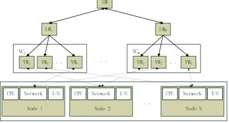
The consolidation scheme proposed in this paper assumes that the Cloud adopts the architecture illustrated in Fig.1.

Multiple VCs, denoted as VC1, VC2, …, and VCM, coexist in

the Cloud system. The Cloud system consists of a cluster of

N physical nodes, n1, n2, …nN. Creating a VM needs to

also often adopted in literature [8][9][12][30][42], in which the most notable example is Eucalyptus [15][42].

Each node has at most one VM of each VC. The reason for limiting this is because the consolidation framework in this paper can adjust the resource capacity allocated to VMs. Therefore, if there is the need to map two VMs from the same VC to the same physical node, it is very likely that we can increase the resource allocation of one VM (according to the performance model) so that the upsized VM has the same processing capability as the total processing capability of

these two VMs. VMij denotes VCj’s VM in node ni. Assume

the capacity of resource ri allocated to a VM in VCj have to

be in the range of [mincij, maxcij]. mincij is the minimal

requirement for resource rj when generating a VM for VCi,

and maxcij is the capacity beyond which the VM will not

gain further performance improvement. For example,

minimal memory requirement for generating a VM in VCj is

50 Megabytes, while the VM will not benefit further by allocating more than 1 Gigabytes of memory. We assume

that the physical nodes are homogeneous. mincij and maxcij is

normalized as a percentage of the total resource capacity in a physical node. It is straightforward to extend our work to a heterogeneous platform.

A VC’s LM can use the existing VM management strategy in literature to create VMs in physical nodes [30], and use existing request scheduling strategy to determine a suitable VM for running an incoming request [30]. The server consolidation scheme is deployed in GM and works with the VM management strategy and the request scheduling strategy in LMs to achieve optimized performance for the Cloud. The server consolidation procedure will be invoked when necessary (the invocation timing will be discussed in Section IV). After the server consolidation is completed, the consolidation procedure will inform LMs of the new system state, i.e., VM-to-node mapping and resource capacities allocated to each VM. LMs can then adjust the dispatching of requests to VMs accordingly.

Figure 1. The hierarchy of the Cloud System

IV. THE GENETIC ALGORITHM

In this work, a VM may consume multiple types of resources. For example, the VC serving CPU-intensive requests will mainly consume CPU cycles while the VC processing I/O-intensive requests needs to consume a large

amount of I/O capacity. It is a NP-hard problem to optimize the consumptions of multiple types of resources. A Genetic Algorithm (GA) has been designed and implemented in this work to compute the optimized system state, i.e., VM-to-node mapping and the resource capacity allocated to each VM, so as to optimize resource consumptions in the Cloud. The GA can work with the existing request schedulers in literature [30], which is deployed in the GM and LMs.

The increase in the arrival rates of the incoming requests may cause the current VMs in the VC cannot satisfy the desired QoS level, and therefore a new VM needs to be created with desired resource capacity.

The invocation of the GA will be triggered if the

following situations occur, which are termed as resource

fragmentation:

1) There are spare resource capabilities in active nodes. An active node is a node in which the VMs are serving

requests. Denoting the spare capability of resource rj in node

ni as scij;

2) The spare resource capabilities in every node are less

than the capacity requirements of the new VM in VCk,

denoted as ckj, i.e.,

For i (1≤i≤N), there exists such j (1≤j≤R), so that scij < ckj

3) The total spare resource capabilities across all used physical nodes are greater than the capacities required by the new VM, i.e.,

For j (1≤j≤R), the following inequality holds, where  is no less than one and used to control the level of spare capability in the Cloud that can trigger the GA. The bigger  is, less frequently the GA will be invoked and to greater extent the resources will be consolidated. The value of  is determined empirically.

kj N

i scij  c



The motivation of invoking the GA is to converge the spare capacity to as few number of nodes as possible so that we can create the new VM in one of the active nodes, and therefore avoid waking up an inactive node.

If the arrival rates of requests decrease, the resource capacity allocated to VMs will become excessive. The deployed request scheduler will re-distribute the requests among VMs. If this redistribution causes a VM becomes idle, the VM may be deleted. If all VMs in a node are deleted, the node can be switched off or enter the sleep mode to save energy. So the decrease in the requests’ arrival rates will not trigger the invocation of the GA. But note the deletion of VMs will generate spare resource capacity in nodes.

Typically, a GA needs to encode the evolving solutions, and then perform the crossover and the mutation operation on the encoded solutions. Moreover, a fitness function needs to be defined to guide the evolution direction of the solutions. In this work, the solution that the GA strives to optimize is the system state, which consists of two aspects: the VM-to-node mapping and the resource capacity allocated to each VM. In this work, a system state is represented using a three dimensional array, S. An element S[i, j, k] in the array is the percentage of total capacity of resource rk in node ni that is

the crossover and mutation operation as well as the fitness function developed in this work.

A. The Crossover Operation

Given a generation of solutions, represented in the S

array, the crossover and mutation operations will be performed in the GA to generate the next generation of solution. The crossover operation takes as input two solutions, called parent solutions, in the current generation of solution set and generates two children solutions using the following method.

Assume there are M VCs in the Cloud, VC1, VC2, ..., VCM.

The resource capacity allocated to VCj is recorded in S[*, j,

*], which is a two dimensional array. Assume that the

resource capacity allocated to VCj in two parent solutions are

S1[*, j, *] and S2[*, j, *] (1≤j≤M), respectively. In the

crossover operation, a VC index p is randomly selected from

the range of 1 to M, and then both of the two parent solutions

are partitioned into two portions at the position of the index p.

Subsequently, the crossover operation merges the head (and tail) portion of parent solution 1 with the tail (and head) portion of parent solution 2, and generates child solution 1 (and 2).

The validity check will be performed in both children solutions to ensure that the total resource capacity allocated to the VMs in a node is not more than the physical resource capacity of that node. This constraint can be expressed as

follows, where R is the number of resource types.

For i, k: 1≤i≤N, 1≤k≤R, [, , ] 1

1 



j Si j k (1)

If there exists q (1≤q≤N) such that Eq.1 does not hold, then

the crossover operation is not performed for node nq.

The crossover operation is designed to consolidate VMs into a smaller number of nodes without adjusting the resource capacities allocated to VMs.

B. The Mutation Operation

After the crossover operation, the mutation operation is then performed over the generated children solutions, aiming to adjust the resource capacity allocated to the VMs to further converge the spare capabilities to a smaller number of nodes. In the mutation operation, the quantity of an element in the matrix S[i, j, k] will be adjusted. So the GA needs to determine which element is adjusted (i.e., determining index

i, j, k). The procedure is as follows.

i) Determining index i, j, k

A VC is first randomly selected (j is determined). Then a

node is selected (i is determined) with the probability

proportional to the capacity of the major resource type

consumed by the selected VC in that node (for the VC which

serves CPU-intensive requests, the major resource type is

CPU). After that, a resource type is selected (k is determined)

with the major resource type having a higher probability of being selected than other resource types. The ratio probability of selecting the major resource type to other resource types are set to be R and 1, respectively (R is the

number of resource types in the system). Assume VCi is

selected, VCi consumes three types of resources and resource

r1 is the major resource type. Then the relative selection

probability for resource r1, r2, and r3 is 3:1:1. The reason of giving a higher probability to select the major resource type is because the major resource type has greater impact on the VM’s processing capability.

ii) Adjusting resource capacities

After determining i, j and k, S[i, j, k] is increased by a quantity randomly chosen from [0, min(maxcjk−S[i, j, k], scik)] (scik is the spare capability of resource rk in node ni). After the adjustment, the GA calculates the increased service rate

in node ni, denoted as . is the service rate that can be

reduced in another VM, say VMqj (qi) and the desired QoS

for VCj can still be satisfied. If there is a VM whose current

service rate is less than , then the resources allocated to

that VM can be reclaimed. If such a VM does not exist, the

capacity of resource rk allocated to VMkj is reduced by a

quantity calculated from the performance model. VMqj is not

randomly selected, but with the probability proportional to 1/S[q, j, k]. The reason for this is that the node with less capacity being allocated to its VM will have higher probability of being selected.

C. The Fitness Function

The fitness function in a GA is used to evaluate the quality of the solutions. In this work, the fitness function is constructed as follows.

Assume the number of active nodes is N and the spare

capacity of a type of resource rk in node ni is scik. Resource

fragmentation can be reduced when the spare capacities converge to a smaller number of nodes. Therefore, the standard deviation of the variables, scik (1iN), can reflect

the convergence level rk’s spare capability across N nodes.

The bigger the standard deviation is, the higher convergence level.

Since multiple types of resources are taken into account in this work, it is desired that the spare capacity of different types of resources converges to the same node. For example, we prefer the case where a node has balanced spare CPU cycles and memory, rather than the case where there is a large amount of spare memory but fully utilized CPU in one node, while a large amount of spare CPU cycles but fully utilized memory in another. The standard deviation of the variables, scik (1kR), can reflect to what extent there are balanced spare capacities across different types of resource

in node ni. The smaller the standard deviation is, the more

balanced capabilities. The standard deviation of the variables,

scik (1kR), in node ni can be calculated using Eq.2, where

s i

sc is the average of scik (1kR) and can be calculated in Eq.3.

R sc sc

R k

s i ik i



 1

2 ) (

 (2)

R sc sc

R k ik s

i



 1 ₍₃₎

The above two factors are combined together to construct the fitness function for the GA, which is shown in Eq.4,

where a

k

N active nodes and can be calculated in Eq.5. In Eq.4, ) , ( s i i sc

W  is a weight function and used to calculate the

weighted sum of the deviation of resource rk’s spare capacity

in multiple nodes. The weight is determined based on the

relation between _i and s

i

sc , which is partitioned into six

bands. Each of the first five bands spans 20% of s

i

sc and the

weight function falls into the last band when i

 is greater

than s

i sc .

 



After a population of solutions is generated, each solution is evaluated by calculating the fitness function. The solution with higher value of the fitness function has higher probability to be selected to generate the next generation of solutions. The GA is stopped after it runs for a predefined time duration or the solutions have stabilized (i.e., does not improve over a certain number of generations).

V. RECONFIGURATING VIRTUAL CLUSTERS

Assume S and S′ are the matrixes representing the system

states before and after running the GA, respectively. The Cloud system needs to reconfigure the Virtual Clusters by

transiting the system state from S to S′. During the transition,

various VM operations will be performed, such as VM creation, VM deletion, VM migration as well as changing a VM’s resource capacities. This section analyzes the transition time and presents a cost model for the Cloud reconfiguration. A reconfiguration algorithm is then presented to determine the reconfiguration plan that has low transition time, therefore imposes the low overhead.

A. Categorizing Changes in System States

The differences between S[i, j, k] and S′[i, j, k] can be categorized into the following cases, which will be handled in different ways.

Case 1: Both S[i, j, *] and S′[i, j, *] are non-zero, but

have different values: this means that the resource capacity

allocated to VMij needs to be adjusted. It can be further

divided into two subcases: 1.1) S[i, j, *] is greater than S′[i,

j, *], which means that VMij needs to reduce its resource

capacity, and 1.2) S′[i, j, *] is greater than S[i, j, *], which

means that VMij needs to increase its resource capacity;

Case 2: S[i, j, *] is non-zero, while S′[i, j, *] is zero: this

means that node ni is allocated to host VCj (i.e., VMij) before

running the GA, but is not allocated to host VCj after. In this

case, there are two options to transit the current system state

to the new one: 2.1) Deleting VMij, and 2.2) Migrating VMij

to another node which is allocated to run VCj after running

the GA;

Case 3: S[i, j, *] is zero, while S′[i, j, *] is non-zero: this

case is opposite to case 2). In this case, the system can either 3.1) Create VMij, or 3.2) accept the migration of VCj’s VM

from another node.

B. Transiting System States

1) VMOperations during the Transition

DL(VMij), CR(VMij), CH(VMij) denote the time spent in completing deletion, creation, and capacity adjustment operation for VMij, respectively. MG(VMij, nk) denotes the time needed to migrate VMij from node ni to nk (i≠k). Note one difference between VM deletion and VM migration. A VM can be deleted only after the existing requests scheduled to run on the VM have been completed, while the VM can continue the service during live migration. The average time

needed for VMij to complete the existing requests, denoted as

RR(VMij), can be calculated as follows.

Assume that the number of requests in VMij is mij,

including the request running in the VM and the requests

waiting in the VM’s local queue. mij can be obtained by

monitoring the status of the queue in the VM.

Assume the average execution time of a request is e, and

the request which is running in the VM has been running for

the duration of e0. Then RR(VMij) can be calculated in Eq.7.

RR(VMij)=(mij−1)×e + (e−e0) (7)

These four types of VM operations can be divided into two broad categories: 1) resource releasing operation, including deleting a VM, migrating a VM to another node, and reducing the resource capacity allocated to a VM; 2) resource allocation operation, including creating a VM, accepting the migration of a VM from another node, and increasing the resource capacity allocated to a VM. When both categories of VM operations need to be performed when reconfiguring a node, careful considerations have to be given to the execution order of the VM operations, because the node may not have enough resource capacity so that resource releasing operations have to be performed first before resource allocation operations can be conducted. Therefore, there may be execution dependencies among VM operations. Below, we first discuss the condition under which there are no execution dependencies among VM operations when reconfiguring a node, and then analyze how to perform VM operations when the condition is or is not satisfied. We also analyze the time spent in completing these operations.

2) Performing VM Operations without Dependency

If total resource capacities of the VMs in a node do not exceed the total physical resource capacity of the node at any time point during the transition, the VM operations in the same node do not have dependency. This condition can be formalized in Eq.8.

For k: 1≤k≤R, max( [, , ], '[, , ]) 1

1 



j S i j k S i j k (8)

i) time for reconfiguring a node without VM migrations

The transition time for reconfiguring node ni, denoted as

TR(ni), can be calculated using Eq.9, where Sdl, Scr and Sch

denote the set of VMs in node ni that are deleted, created and

adjust their resource allocations during the reconfiguration, respectively; The second term in the equation (i.e. the term

within the min operator) reflects the reality that the activities

of creating a new VM and adjusting a VM’s resource capacity can be conducted at the same time as executing the existing requests in the VMs to be deleted.







ii) time for reconfiguring a node with VM migrations

If the reconfiguration of node ni involves VM migrations,

including ni migrating a VM to another node and ni accepting

a VM migrated from another node, we introduce a concept of

mapping node of ni, which is further divided into mapping

destination node, which is the node that the VM in ni

migrates to, and mapping source node, which is the node that

migrates a VM to ni. When handling VM migrations in ni,

ni’s mapping node will be first identified as follows. If the

following two conditions are satisfied, node nq (i≠q) can be a

mapping destination node of node ni, and node ni is called

nq’s mapping source node.

 k, 1≤k≤R, S[i, j, k] > 0, but for k, 1≤k≤R, S[i, j, k]=0  For k, 1≤k≤R, S[q, j, k]=0, but k, 1≤k≤R, S[q, j, k] > 0

Note that a node can have multiple mapping nodes. Which mapping node is finally selected by the reconfiguration procedure will have impact on the transition time.

If ni accepts a VM migration from nq during the

reconfiguration of ni, then the time for reconfiguring ni can

be calculated from Eq.10, where Smg denotes the set of VMs

in node ni that are migrated from another node.

}} | ) ( max{ , ) ( ) ( ) , ( min{ ) ( ) ( dl ij ij S VM ij S VM ij S VM k ij S VM ij i S VM VM RR VM CH VM CR n VM MG VM DL n TR ch ij cr ij mg ij dl ij     









If ni migrates a VM to another node, the reconfiguration

procedure will check whether Eq.8 holds for ni’s mapping

destination node. If Eq.8 holds, then the VM can be migrated to that node at any time point. Otherwise, the VM migration will be handled in a different way, which is presented in Section V.B.3.

When Eq.8 holds for ni, the reconfiguration procedure of

ni is outlined in Algorithm 1. Step 5-7 of the algorithm deal

with VM migrations, which will be discussed in detail in Section V.B.3. Note that Case 3 is not handled in this algorithm. The reason for this will be explained when Algorithm 4 is introduced.

Algorithm 1. Reconfiguration_without_dependency(ni);

1. for each VMij in Case 1 do

2. Adjust the resource capacity of VMij;

3. for each VMij in Case 2.1 do

4. Delete VMij;

5. for each VMij in Case 2.2 do

6. Find a mapping destination node, nk, for the VM,

denoted as VMij; 7. Call migration(VMij, nk); 8. return;

3) Performing VM Operations with Dependency

If Eq.8 does not hold, there must be at least one VM in the node which releases resources during the reconfiguration. Otherwise, if all VMs in the node only acquire resources and Eq.8 does not hold, the resource capacity allocated to the VMs in the node will exceed the node’s physical resource capacity after the reconfiguration.

A VM can release resources by the following three possible operations during the reconfiguration:

 Reducing the resource capacity allocated to the VM,

 Deleting the VM,

 Migrating the VM to another node.

If there are multiple VMs releasing their resources in

node ni, the reconfiguration procedure will release resources

in the above precedence, until Eq.5.3 satisfies, where S[i,j,k]

is now the current resource capacity allocated to the VMs in the node after the resources have been released so far. Once Eq.8 holds, it indicates the remaining reconfiguration process can be conducted using the way discussed in Subsection V.B.2. If multiple VMs perform the same type of resource releasing operations, a VM with the greatest amount of capacity to be released will be selected.

The end of Subsection V.B.2 mentioned the situation

where ni tries to migrate a VM to a mapping node, but Eq.8

may or may not hold for that node. The procedure of

migrating VMij to node nk is outlined in Algorithm 2, which

is called in Algorithm 1 (Step 7). The algorithm will first check whether Eq.8 holds for the mapping node (Step 1). If it holds, the VM migrates to the mapping node straightway (Step 21). If it does not hold, the VM migration operation does have dependency and some resource releasing operations have to be completed in the listed precedence (Step 2-19) until Eq. 8 holds. Under this circumstance, the algorithm becomes an iterative procedure (Step 16) and resource releasing operations will be performed in a chain of nodes.

Algorithm 2. migration(VMij, nk) //migrating VMij to nk 1. if Eq.5.3 does not hold for nkthen //with dependency 2. for each VMkj in Case 1.1 do

3. reduce VMkj’s resource allocations and update

S[k, j, *] accordingly;

4. if Eq.5.3 holds then

5. migrate VMij to nk and update S[k, j, *]

and S[i, j, *] accordingly;

6. return;

7. end for

8. for each VMkj in Case 2.1 do

9. delete VMkj and update S[k, j, *] accordingly;

10. if Eq.5.3 holds then

11. Migrate VMij to nk and update S[k, j, *]

and S[i, j, *] accordingly;

12. return;

14. for each VMkj in Case 2.2 do

15. Obtain a mapping node, nq;

16. Call migration(VMkj, nq);

17. If Eq.5.3 holds then

18. Migrate VMij to nk and update S[k, j, *] and S[i,

j, *] accordingly;

19. return;

20. else //without dependency

21. migrate VMij to nk and update S[k, j, *] and S[i,

j, *] accordingly;

22. return;

Algorithm 3 is used to reconfigure node ni. In the

algorithm, if Eq.5.3 does not hold for ni, the resources will be

released until Eq.5.3 satisfies. Then Algorithm 1 is called to reconfigure the node (Step 16).

Algorithm 3. Reconfiguration(ni)

1. if Eq.5.3 does not hold then //with dependency 2. for each VMij in Case 1.1 do

3. reduce VMij’s resource allocations and update

S[i, j, *] accordingly;

4. if Eq.5.3 holds then break;

5. end for

6. for each VMij in Case 2.1 do

7. delete VMij and update S[i, j, *] accordingly;

8. if Eq.5.3 holds then break;

9. end for

10. for each VMij in Case 2.2do

11. Obtaining the mapping node, nk;

12. Call migration(VMij, nk);

13. if Eq.5.3 holds then break;

14. End for

15. End if

16. call Reconfiguration_without_dependency(ni);

17. return;

Algorithm 4 is used to construct the reconfiguration plan for the Cloud. Note that the VMs in Case 3 are handled in this algorithm (Step 7-9) by creating the VMs. This is

because when migrating VMij from node ni to the mapping

node nk, Case 3 has been handled for VMkj in node nk (Case

3.1). Therefore, when Algorithm 4 completes Step 2-6, the VMs that are left unattended are those which were not used as the mapping destination nodes for VM migrations. The only option to deal with those VMs now is to create them. Algorithm 4. Reconfiguring the Cloud

Input: S[i, j, k]

1.  = the set of all nodes in the Cloud;

2. while ( ≠ )

3. Obtain node ni (1≤ i ≤N) from ;

4. Call Reconfiguration (ni);

5.  = ni;

6. end while

7. for each node, ni do,

8. for each VMij in Case 3 that has not been handled do

9. Create VMij;

C. Calculating Transition Time

A DAG graph can be constructed based on the dependencies between the VM operations as well as between source nodes and mapping destination nodes. As can be seen

in Algorithm 3, if Eq.8 does not hold for ni, the VM

operations have to be performed in a particular order, which causes the dependency between VM operations. Also in

Algorithm 2, if migration(VMkj, nq) is further invoked during

the execution of migration(VMij, nk), then there is the

dependency between node nq and nk. This is because nk

depends on nq releasing resources before a VM in nk can

migrate to nq.

In this paper, a DAG graph is used to model the dependency between nodes. In the DAG graph, a node

represents a physical node, and an arc from node ni to nk

represents a VM migrating from nk to ni. A case study is

illustrated in Fig.2. Assume there are four VCs (VCj, 1≤j≤4)

in the Cloud. Each node has at most four VMs, each

belonging to a different VC. Assume n1 has all four VMs and

n2 has VM21 (the VM belonging to VC2) and VM24 (the VM

belonging to VC4) before running the GA. After running the

GA, n1 has VM11 and VM14 while n2 has VM22 and VM23. The

resource capacity of VM11 after running the GA is less than

that before running the GA, while the resource capacity of

VM14 after running the GA is greater than that before. The

VM distributions in node n1 and n2 before and after running

the GA can be encoded as in Table I, where 1- and 1+ stand

for the reduced and increased capacity, respectively, compared with before running the GA.

TABLE I. VM MAPPING BEFORE AND AFTER RUNNING THE GA

n1 n2

Before 1 1 1 1 1 0 0 1

After 1- 0 0 1+ 0 1 1 0

The case study further assumes Eq.8 does not hold for n1..

Therefore n1 has to release the resources capacity of VM11,

VM12 and VM13 before VM14 can increase its resource

capacity. Assume in the current reconfiguration plan, VM12 is

to be deleted and VM13 to be migrated to n2 (assume n2 is the

mapping destination node). Assume Eq.8 does not hold for

n2 either, and VM21 has to migrate to n3 and VM24 migrate to

n4 before VM22 and VM23 can be created in n2.

Figure 2. A case study of node dependency during the reconfiguration

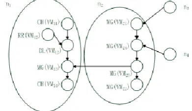
Based on the above assumptions, VM operations in n1

and n2 as well as their dependencies are as follows.

sequence of the VM operations in n1 is: 1) VM11 reduces its

resource capacity; 2) VM12 is deleted; 3) VM13 is migrated to

n2. Operation 1) can occur anytime. Operation 2) can occur

only after the existing requests in the VM have been

completed. Operation 3) depends on VM21 and VM24

releasing resources, since the creation of VM23 can only be

performed after VM21 and VM24 have been migrated. The

migrations of VM21 and VM24 further depend on resource

releasing operations in n3 and n4, respectively. The chain of

dependencies continues until Eq.8 holds for n5, which means

that the VMs in n3 and n4 can migrates to n5 freely and do not

depend on other VM operations in n5. The dependencies

between the VM operations in different nodes can also be modeled as a DAG graph. The dependencies between VM operations in n1 and n2 can be illustrated in Fig.3.

Figure 3. The dependencies between the VM operations in n1 and n2

If the VM operations in all nodes form a single DAG, calculating the transition time of the reconfiguration plan for the Cloud can be transformed to compute the critical path in the DAG. The VM operations involved in reconfiguring the Cloud may also form several disjoint DAG graphs. In this case, the critical paths of all these DAG graphs need to be computed. The time of the longest critical path is the transition time of the reconfiguration plan for the whole Cloud since the VM operations in different DAG graphs can be performed in parallel.

There can be different reconfiguration plans and different plans may have different transition times. The uncertainty comes from two aspects: 1) which of the two VM operations, deletion or migration, should be performed for a VM in Case 2, and 2) if a VM is to be migrated and it has multiple mapping destination nodes, which node should be selected to migrate the VM to. More specifically, before invoking Algorithm 3, we need to decide for all VMs in Case 2, which VMs should be classified into Case 2.1 (relating to Step 6 of Algorithm 3) and Case 2.2 (relating to Step 10). Moreover, in Step 11, the system needs to determine which mapping node should be selected. The objective is to obtain a reconfiguration plan which has the low transition cost. We now present the strategies to find such a plan.

An approach to obtaining the optimal reconfiguration plan is to enumerate all possibilities for each VM falling into Case 2, i.e., to calculate the transition cost for both Case 2.1

and Case 2.2. If there are k VMs which fall into Case 2, then

there are 2k combinations of delete/migration choices and the

transition cost for each combination needs to be calculated.

After determining to migrate a VM, another uncertainty is that the VM may have multiple mapping nodes. Suppose

VMij has pj mapping nodes. We need to enumerate all

possibilities and calculate the transition cost pj times for

migrating a VM to each of its pj mapping nodes. Each

possibility corresponds to a DAG. Therefore, the enumeration approach will examine all these different DAGs. The DAG with the shortest critical path represents the optimal reconfiguration plan.

Apparently, the time complexity of the enumeration approach is very high. We developed a heuristic approach to obtain a sub-optimal reconfiguration plan quickly. The strategies used in the heuristic approach are as follows.

a) determining deletion or migration:

D(VMij) denotes the time the system has to wait for

completing the deletion of VMij. As discussed in subsection

V.B.1, D(VMij)=DL(VMij)+RR(VMij). If the following two

conditions are satisfied, VMij is migrated. Otherwise, VMij is

deleted.

i) VMij has at least one mapping node such that migrating

VMij to that node will not trigger other VM deletion or

migration operations.

ii) For all mapping nodes satisfying the first condition, there exists such a node, nk, that D(VMij) > MR(VMij, nk)

The two conditions try to compare the time involved in deleting and migrating a VM. Before invoking Algorithm 3 in subsection V.B.3, these two conditions will be applied to determine whether a VM in Case 2 should be handled as Case 2.1 (Step 6) or Case 2.2 (Step 10)

b) determining the mapping node

If a VM is to be migrated and there are multiple mapping destination nodes which satisfy condition ii), then Step 11 of Algorithm 3 will select the node which offers the shortest migration time MR(VMij, nk).

VI. EXPERIMENTAL STUDIES

In this section, we first present the results of the simulation experiments to show the effectiveness of the GA and the Cloud reconfiguration method presented in this paper, and then we present the experimental results of deploying the implementation of CFMV on a real 16-node cluster.

A. Simulation Experiments

A discrete event simulator has been developed to evaluate 1) the performance of the developed GA in consolidating resources, 2) the time spent by the GA in obtaining the optimized system state, and 3) the transition time of the reconfiguration plan obtained by the enumeration approach and the heuristic approach.

In the experiments, three types of resources are simulated: CPU, memory and I/O, and there are three types of VMs: CPU-intensive, Memory-intensive, and I/O-intensive VMs. A VC consists of the same type of VMs. For the CPU-intensive VMs, the required CPU utilisation is selected from the range of [30%, 60%], while their memory and I/O utilisation are selected from the range of [1%, 15%]. The

selection range represents [mincij, maxcij] discussed in

allocated memory is selected from the range of [30%, 60%], while their CPU and I/O utilisation are selected from the range of [1%, 15%]. For the I/O-intensive VMs, the required I/O utilisation is selected from [30%, 60%], while their CPU and the memory utilisation are from the range of [1%, 15%].

N is the number of physical nodes in the cluster, M is the

number of virtual clusters in the Cloud, f is the percentage of

the spare capability in a node.

The initial VM-to-node mapping is generated in the following manner.

i) Set the number of VMs in a node is b (b is set to be 3

in the simulation experiments, unless otherwise stated); ii) Use the resource selection ranges above to generate

b*N/3  computation-intensive VMs, b*N/3 for

memory-intensive VMs, and (b*N – 2*b*N/3) I/O-intensive VMs;

iii) Calculate the average size of the VCs (i.e., the

number of VMs in a VC) as b*N/M;

iv) Use the first fit algorithm [34] to generate the initial

VM-to-node mapping, i.e, for VMij, search the nodes starting

from n1, if the node has enough capacity (after deducting the

f spare capability) to accommodate VMij, then map VMij to

the node.

GA takes as input the initial system state generated as above and calculates an optimized state.

Other experimental settings are detailed in individual experiments.

Representative times in the literature [34][39] were assumed in our simulation experiments. The average time for deleting and creating a VM is 20 and 14 seconds, respectively. The migration time depends on the size of VM image and the number of active VMs in the mapping nodes [34][39]. The migration time in our experiments is in the range of 10 to 32 seconds.

1) Performance of the GA

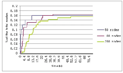
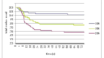
a) Impact of the Number of Physical Nodes

Fig.4 shows the number of nodes saved as the GA progresses. In the experiments in Fig.4, the number of nodes with active VMs varies from 50 to 200. The experiments aim to investigate the time that the GA needs to find an optimized system state, and also investigate how many nodes the GA can save by converging spare resource capacities. The free capacity of each type of resource in the nodes is selected randomly from the range [10%, 30%] with the average of 20%. The number of the VMs in a physical node is 3. The number of the VCs in the system is 30. As can be observed from Fig.4, the percentage of nodes saved increases as the GA runs for longer, as to be expected. Further observations show that under all three cases, the number of nodes saved increases sharply after the GA starts running. It suggests the GA implemented in this paper is very effective in evolving optimized states. When the GA runs for longer, the increasing trend tides off. This is because that the VM-to-node mapping and resource allocations calculated by the GA approaches the optimal solutions. Moreover, by observing the difference of the curve trends under different number of nodes, it can be seen that as the number of nodes increases, it takes the GA longer to approach the optimized state. For example, when the number of nodes is 50, the optimized

solution is almost reached after the GA runs for about 13 seconds, while it takes the GA about 53 seconds to reach the optimized solution when the number of nodes is 200.

Figure 4. The quantity of nodes saved as the GA progresses

0 8 16 24 32 40 48 56 64 72 80

50 100 200

The number of active nodes

T

im

e s

p

ent

in

fi

nd

in

g op

timi

z

ed

s

y

s

tem

s

ta

te

s

(s

e

c

.)

GA

GA w ith only mutation

Figure 5. Resource consolidation by the GA with only mutation operations; the experimental settings are the same as in Fig.4.

0 0.02 0.04 0.06 0.08 0.1 0.12 0.14 0.16 0.18

10 30 50 70 90 110 130 150 170 190 t he n um b e r o f n o d es

t

h

e

p

r

o

p

o

r

t

i

o

n

o

f

n

o

d

e

s

s

a

v

e

d

GA entropy

Figure 6. The comparison between the GA and entropy; the average free resource capacity is 20%

could still find optimized system states. However, the GA performing only mutation operations had to spend much longer time to reach the optimized states. Fig.5 compares the time spent by the GA performing both crossover and mutation operations with the time by the GA only performing mutations. The experimental settings are the same as in Fig.4. As can be seen from this figure, under all experimental settings, the time spent by the GA performing only mutations is significantly longer. These results can be explained as follows. The crossover operation essentially tries to find a better way to pack the VMs into physical nodes. Without the crossover operation, although mutation operation can also eventually achieve the same effect by adjusting resource capacities of individual VMs, the process would be much longer. This is because the mutation operation is performed on a single VM each time, while the crossover operation is performed on a set of VMs.

Fig.6 compares the GA developed in this work with the Entropy consolidation scheme presented in [34]. It can be seen from this figure that the GA clearly outperforms Entropy in all cases. This is because the VMs’ resource allocations in Entropy remain unchanged, while the GA developed in this paper employs the mutation operation to adjust the VMs’ resource allocations. This flexibility makes the VMs “moldable” and therefore is able to squeeze VMs more tightly into fewer nodes. It can also been observed from this figure that there is no clear increasing or decreasing trend in terms of the proportion of nodes saved as the number nodes increases in our consolidation scheme. This suggests that the number of nodes does not have much impact on the GA’s capability of saving nodes.

Figure 7. The impact of free resource capacity in nodes on the performance of GA; the initial number of nodes used are 200; the number of the Virtual Clusters in the system is 30;

b) Impact of Free Capacity

Fig.7 demonstrates how the GA performs under different level of free capacity in the physical nodes. In the experiments presented in Fig.7, the number of the VCs in the system is 30 while the free capacity of the resources in each node varies from 10% to 20%. It can be observed from this figure that the number of nodes used to host the VCs decreases as the level of free capacity increases. This result demonstrates the effectiveness of the developed GA in exploiting the free resources to consolidate the VMs into a smaller number of nodes. It can also be seen from the figure that although the time that the GA spends to approach the

optimal solution increases as the level of free capacity increases, the increase is moderate (not as big as when the number of nodes increases). When the level of free capacity increases from 10% to 20%, the time the GA takes to almost reach the optimized solution increases from 22 seconds to 27 seconds. This result suggests that the level of free capacity in the nodes does not have big impact on the running time of the GA.

c) Impact of the Number of VCs

Fig.8 shows how the GA performs under different number of VCs. In this figure, the total number of VMs in the Cloud is fixed to be 600, while the number of VCs varies from 20 to 40. When the number of VCs in the Cloud is 20, 30 and 40, the average number of VMs that each VC has is 30, 20 and 15, respectively. As seen from this figure, the number of nodes used to host the VCs decreases in all cases as the GA progresses, which is to be expected. It can also be observed that the time that the GA spends to approach the optimized solution becomes longer as the number of VCs increases. When there are 20 and 40 VCs, for example, the GA takes 17 and 52 seconds, respectively, to achieve the near-optimal solution. Another observation is that although the free resource capacity is 20% in all cases, the final number of consumed nodes calculated by the GA is different under different number of VCs. As observed from the figure, the number of consumed nodes decreases as the number of VCs in the Cloud increases. This result can be explained as follows. According to the experimental settings in the figure, when there are more VCs, the granularity of a VC in terms of the number of VMs is smaller. Therefore, the GA has more opportunities to consolidate the VCs into a smaller number of nodes. This result shows that the number of VCs has the mixed impact on the GA’s performance. When more VCs are hosted, a longer time may be taken to reach the optimized solution, but potentially more resources may be saved. This gives the insight into how to determine a suitable number of VCs in a Cloud, given a certain number of underlying physical nodes.

Figure 8. The impact of the number of VCs on the performance of the GA; the number of physical nodes is 200; the average level of free resource capacity in nodes in 20%.

2) Performance of the Cloud Reconfiguration