Antenna aperture phase retrieval

(1)

ANTENNA APERTURE PHASE RETRIEVAL

Peter H. Gardenier

A thesis presented for the degree of

(2)

(3)

ABSTRACT

Geometrical defects of a high gain reflector antenna can cause the radiation pattern of the antenna to fail to meet its specifications. These defects give rise to loss of gain, widening of the main beam and raising of sidelobes. The geometrical defects can be identified, and subsequently corrected, by utilizing information contained in the phase of the copolar aperture field distribution. For technical reasons, this phase can be difficult or inconvenient to measure directly. Therefore, indirect methods of deducing the phase are often preferred.

This thesis introduces an iterative algorithm, called the modified Gerchberg-Saxton algori thm, which has been developed for retrieving the copolar aperture field phase distribution from the far field copolar amplitude pattern. In order to aid convergence of this algorithm, it incorporates information concerning the design and any known aspect of the antenna. The modified Gerchberg-Saxton algorithm is based on the conventional Gerchberg-Saxton algorithm, originally developed for electron microscopy, but incorporates features of Fienup's phase retrieval algorithms.

This thesis reviews radio engineering theory with an emphasis on high gain reflector antennas. In particular, the Fourier transform relationship between the copolar aper-ture field distribution and the copolar radiation pattern is critically examined. The problem of retrieving the copolar aperture field distribution from the amplitude of its Fourier transform is called a Fourier phase problem. The Fourier phase problem, the uniqueness of its solutions and iterative algorithms for solving it are discussed. Other established methods for determining geometrical defects of an antenna are descri bed and their relative advantages and disadvantages are assessed. The main advantage of the modified Gerchberg-Saxton algorithm is that it requires measurement of only a single copolar amplitude pattern.

(4)

(5)

ACKNOWLEDGEMENTS

The research for my Ph.D. project and the writing of this thesis could not have come about if it was not for the support of many people. I am especially grateful to my supervisor Professor Richard Bates, for his much valued guidance and encouragement during the course of my research, and for the enormous amount of time and effort he has spent in edi ting this thesis.

The Telecom Corporation of New Zealand Limited (formally the New Zealand Post Office) has provided me with financial assistance for which I am grateful. I thank Drs Murray Milner and Eric Hamilton, both formally with the International Section of the NZPO Headquarters, for their encouragement and for the helpful discussions we had about practical aspects of setting up and operating earth station satellite antennas.

I am grateful for the cooperation of fellow students, academic staff, technical staff and librarians at the University of Canterbury. I have enjoyed the stimulating discus-sions with these people and have learned much from them. Special thanks to Charles Parker, Lim Ching Aun, Michael Cusdin, Wiktor Mencel, Quek Bek Kim and Steve Gunn, all of whom have worked with me on aspects of the research described in this thesis.

(6)

(7)

29

30 30 30 33 34 35 36

37

39

39 40 46

47

48 48 48 51 51 52

53

55

55 56 57 57 58

CHAPTER 3 RETRIEVAL

61

62 3.1 Geometrical defects of reflector antennas

3.2 Relating geometrical defects to aperture phase deviations 64

3.2.1 Reflector shape defects 64

3.2.2 Feed displacement 66

3.2.3 Inferring geometrical defects from aperture phase

deviations 68

3.3 Measurement methods 69

3.3.1 Measurement of reflector shapes 70

3.3.2 Near field scanning techniques 72

3.3.3 Measurements of the Fourier Fresnel and far fields 74

3.3.3.1 Amplitude measurements 74

3.3.3.2 Complex holography 77

3.3.4 Comparison of the measurement methods 82 3,4 Phase retrieval from Fourier transform amplitude 85

(9)

CONTENTS

CHAPTER 4

lX

3.4.1.1 Compact images 86

3.4.1.2 Sampling 88

3.4.1.3 Interpolation and aliasing 88

3.4.1.4 The discrete Fourier transform (DFT) 93 3.4.2 Uniqueness of the Fourier phase problem ~6

3.4.2.1 The Fourier transform amplitude 07

3.4.2.2 The z-transform 98

3.4.2.3 Solutions to the Fourier phase problem 100 3.4.2.4 Images in one and two dimensions 102 3.4.3 Iterative Fourier transform algorithms 103 3.4.3.1 The Gerchberg-Saxton algorithm 105 3.4.3.2 A variant of the Gerchberg-Saxton

algorithm 106

3.4.3.3 Fienup's algorithms 3.5 Phase retrieval in antenna practice

3.5.1 Davis'method

108 115 116 117 120 122 123 124 3.5.2 Amplitude holography

3.5.3 The Misell algorithm

3.5.4 Plane-to-plane diffraction algorithm 3.5.5 Comparison of methods

3.5.6 Far field extrapolation 3.6 Summary

THE MODIFIED GERCHBERG-SAXTON

ALGORITHM: EVALUATION

COMPUTER

SIMULATION.

4.1 Practical implications of the algorithm 4.1.1 Procedure

4.1.2 Ambiguities

4.2 Computer modelling of reflector antennas 4.2.1 Design fields

4.2.2 Field deviations

4.2.3 Measurement inaccuracies 4.2.4 Depolarization

4.3 Error measu res

4.4 The modified Gerchberg-Saxton algorithm 4.4.1 Error reduction algorithms

4.4.2 The CC algorithm 4.4.3 The RIO algorithm

4.4.4 Choice of starting aperture distribution 4.4.5 The composite algorithm

4.4.6 Alternative forms of the modified Gerchberg-Saxton algorithm 4.4.6.1 Local well avoidance

4.4.6.2 The phase relaxation algorithm 4.4.6.3 Constraints involving thresholds 4.4.6.4 Another input-output algorithm 4.5 A worked example

(10)

x CONTENTS

4.6 Relationships between error measures 181 4.7 Far field measurement considerations 183

4.7.1 Smoothing far field data 183

4.7.2 Need for oversampling the far field 186

4.7.3 Truncated far field data 190

4.7.3.1 Direct application of the composite

algorithm 190

4.7.3.2 Extrapolating the far field data 192 4.7.3.3 The extrapolating composite algorithm 192 4.7.3.4 Comparison of approaches to dealing

with truncated data 193

4.8 Assessment of composite algorithm 194

4.8.1 Relatively simple computer models 194 4.8.2 Variations of the basic model 203 4.8.3 Relatively comprehensive computer models 206

4.8.4 Summary of results 208

4.9 Other uses of the modified Gerchberg-Saxton algorithm 209

4.9.1 Estimation of depolarization 209

4.9.2 Aperture amplitude estimation 214

4.10 Summary 219

CHAPTER 5 EXPERIMENTAL VERIFICATION OF MODIFIED GERCHBERG-SAXTON ALGORITHM USING AN

ACOUSTIC ANTENNA 221

5.1 Acoustic waves 221

5.2 Experimental apparatus 225

5.2.1 The antenna 226

5.2.2 Measurement hardware 229

5.2.3 Measurement software 230

5.3 Results 233

5.3.1 Details of two measurements 233

5.3.2 Methods for processing far field amplitude data 235 5.3.3 Methods for evaluating results 236 5.3.4 Processing the far field data 239 5.3.5 Applying the modified Gerchberg-Saxton algorithm 242 5.4 Summary

CHAPTER 6 CONCLUSIONS AND SUGGESTIONS FOR FUTURE WORK

247

249

6.1 Suggestions for future work 249

REFERENCES

6.1.1 Improvements to the modified Gerchberg-Saxton

algorithm 249

6.1.2 Verification of the algorithm 6.1.3 One-dimensional phase retrieval 6.2 Conclusions

(11)

CONTENTS

GLOSSARY

INDEX

Xl

(12)

(13)

PREFACE

An important way in which engineering science can progress is to take ideas developed for one discipline and to apply them to another discipline. For such an application to suggest itself, the two disciplines must share something in common. My supervi-sor, Professor R.H.T. Bates, is in a good position to initiate such inter-disciplinary work because he has a diverse range of interests, many of which revolve around the Fourier transform [Bates, 1987a ; 1987b]. His research group in the Department of Electrical and Electronic Engineering at the University of Canterbury has, for the last two decades, been actively researching in areas including general inverse problems (no-tably computed tomography and ultrasonic imaging), theory and application of image processing, radio antenna engineering and various aspects of biomedical engineering.

I first worked under Professor Bates when I undertook my final year project (for the Bachelor of Electrical and Electronic Engineering degree), which was co-supervised by Professor Bates' research student Alastair Sinton. My project was to investigate a claim by Panarella and Guty [Panarella and Guty, 1983; Panarella, 1985] that optical interference effects reduce at low light levels. If substantial, this claim would have important consequences for radio communications, amongst other things, because the implication appears to be that antenna sidelobes would disappear for very faint signals. The results of experiments that I performed contradicted the claim [Sinton et al., 1986].

This work introduced me to the theory and practice of diffraction and interference effects of electromagnetic waves.

I started my Ph.D. research course, under the supervision of Professor Bates, by working on two projects. The first project involved the problem of determining the depolarization of a high gain reflector antenna from measurements made with a source antenna which itself suffers from an unknown amount of depolarization. A standard method for solving this problem involves physically rotating the high gain reflector antenna, or its feed, by 900 _{about its axis. It is preferable, however, to be able to}

dispense with such physical manipulation of the antenna. It was felt that some kind of holographic-type approach, such as had earlier been applied to the radio engineering phase problem (Sec. 3.5.2), might be helpful. However, after studying the problem for a while, no solution suggested itself to me.

(14)

ori-XlV PREFACE

entation, magnification and brightness of the object [McCallum

et

at,

1986] and,in general, is also uniquely invertible [Gardenier et al., 1986a].

While I was working on the above-mentioned projects, Professor Bates and one of his research students, David Tan, were supervising the final year project of Lim Ching Aun. This project was a preliminary study of the potential usefulness for the radio engineering phase problem of the Gerchberg-Saxton algorithm (Sec. 3.4.3.1), which was originally developed for electron microscopy. I continued this work and my development of it forms the basis of this thesis. Lim Ching Aun later completed a Master of Engineering degree for which he studied how the Gerchberg-Saxton algorithm (that had by then been modified by myself) can be applied to determine the causes of depolarization of a high gain reflector antenna (assuming that the source antenna does not itself suffer from depolarization). An adapted version of this work is reported in Section

4.9.1-The radio engineering phase problem, mentioned in the previous paragraph, in-volves determining an antenna's copolar aperture field distribution when given only the amplitude of its copolar radiation pattern. The radio engineering phase problem often arises for high gain reflector antennas whose copolar phase patterns are difficult to measure. The reason for wanting to determine the copolar aperture field distribution is that its phase provides valuable information about those geometrical defects of the antenna which must be corrected before the antenna can perform optimally. I have developed a modified form of the Gerchberg-Saxton algorithm suitable for solving the radio engineering phase problem. In this thesis it is demonstrated, on the basis of results of computer simulations and an experiment with an acoustic antenna, that this modified Gerchberg-Saxton algorithm provides a potentially practicable method of re-trieving the copolar aperture field phase distribution from a single measured amplitude pattern (hence the title of this thesis: antenna aperture phase retrieval).

This thesis is. written in six chapters. Each chapter concludes with a summary of the main points raised in that chapter. A chapter by chapter outline of the thesis now follows.

Chapter 1 provides an overview of antenna engineering. The fundamentals of elec-tromagnetic wave theory are introduced and the main types of antenna are briefly described. The chapter also discusses the electrical properties of antennas and the ways in which radio waves propagate through the earth's atmosphere.

Chapter 2 concentrates on high gain reflector antennas. Different methods for analysing the scattering from reflectors are introduced. This leads to the derivation of the Fourier transform relationship between the copolar aperture field distribution and the copolar far field pattern. This relationship is of central importance for the modified Gerchberg-Saxton algorithm. Different configurations of reflector antennas are described. Relevant characteristics of the radiation pattern of a high gain antenna are discussed, with particular emphasis on the degradation of the radiation pattern that occurs when the copolar aperture field phase distribution is distorted by geometrical defects of the antenna. The chapter also mentions typical applications for high gain reflector antennas.

(15)

nec-PREFACE xv

essary to solve the radio engineering phase problem (defined earlier in this preface). The radio engineering phase problem is a specialization of the Fourier phase problem. The Fourier phase problem is discussed in detail and it is shown that, in general, it has a unique solution in two dimensions. Existing ways of solving both the Fourier phase problem and the radio engineering phase problem are outlined.

In Chapter 4 the modified Gerchberg-Saxton algorithm is developed. The chapter starts by suggesting ways in which the algorithm could be applied in practice. A generalized computer model of a high gain reflector antenna and the measurement process is then defined .. This model is invoked to generate a wide variety of data to which the modified Gerchberg-Saxton algorithm can be applied. The results of applying the algorithm to many different computer generate data are presented, evaluated and discussed.

In Chapter 5 the modified Gerchberg-Saxton algorithm is applied to data obtained by measuring the amplitude pattern of a sonic antenna. It is shown that the radiation pattern and the aperture field distribution of a sonic antenna are related by the Fourier transform relationship. The apparatus with which the amplitude pattern is measured is described. This chapter also argues that the modified Gerchberg-Saxton algorithm can be usefully applied to data other than those obtained from high gain reflector antenna patterns.

In Chapter 6 a number of avenues for future research are discussed. This chapter and the thesis concludes with a summary of the main features of the modified Gerchberg-Saxton algorithm.

My original research constitutes most of the material described in Chapters 4 and 5. Almost all of the software implementing the modified Gerchberg-Saxton algorithm and the computer model was written by me. This software was written to interface to the improc (image processing) utility which was principally developed by Richard Lane, who is another of Professor Bates' former research students. Most of the electronics for the acoustic experiment were built by Wiktor Mencel, under the supervision of Michael Cusdin. My fellow research student Charles Parker's first project, under Professor Bates' supervision, was to assist me with the measurements. He perfected the mea-surement technique, which he has now incorporated into his own research programme.

Papers and presentations prepared during the course of my Ph.D. research are listed below.

SINTON, A.M., GARDENIER, P.R. and BATES, R.H.T. (1986), 'Reinvestigation of optical interference at low light levels', Speculations in Science and Technology, Vol. 9, No.4, November, pp. 269-278.

McCALLUM, B.C., GARDENIER, P.H. and BATES, R.H.T. (1986), 'Invertible invariant trans-formations for robotic catalogues', in Proceedings of the International Conference on Fu-ture Computing Systems, Christchurch, New Zealand, February, pp. 151-158.

GARDENIER, P.R., McCALLUM, B.C. and BATES, R.H.T. (1986a), 'Fourier transform mag-nitudes are unique pattern recognition templates', Biological Cybernetics, Vol. 54, No.6, September, pp. 385-39l.

GARDENIER, P.B., LIM, C.A., TAN, D.G.H. and BATES, R.H.T. (1986b), 'Aperture distribu-tion phase from single radiadistribu-tion pattern measurement via Gerchberg-Saxton algorithm',

Electronics Letters, Vol. 22, No.2, January, pp. 113-115.

(16)

XVI PREFACE

BATES, R.B.T., FRIGHT, W.R. and GARDENIER, P.R. (1987), 'Gerchberg-Saxton phase retrieval when image magnitude given only approximately', in IDELL, P.S. (Ed.), Digital Image Recovery and Synthesis, ProceedingB of the SPIE Volume 828, August, pp.

171-176.

MILNER, M.O., GARDENIER, P.R. and BATES, R.H.T. (1987), 'Antenna aperture phase from far field magnitude', in IEEE/ AP-S International Symposium and URSI Radio

Science Meeting, Virginia Tech, Blacksburg, Virginia, USA, June.

GARDENIER, P.H., LIM, C.A. and PARKER, C.R. (1988), 'Satellite communications antenna misalignments inferred from far field magnitude', in Proceedings of the 25th New Zealand

(17)

CHAPTER 1 OVERVIEW

OF

ANTENNA ENGINEERING

The existence of radio waves was confirmed just over 100 years ago by Hertz [O'Hara and Pricha, 1987]. Since then, these waves have become an integral part of modern life. The world has been transformed by radio, and even more by television.

This chapter provides a brief overview of antenna engineering. Section 1.1 intro-duces the theory of electromagnetic waves (of which radio waves are a subset), starting with Maxwell's equations. Radio waves are transmitted and received by antennas. The properties and different types of antennas are summarized in Sections 1.2 and 1.3. The effects on radio wave propagation of the earth and its atmosphere are discussed in Sec-tion 104. This chapter concludes with a summary of important practical applications of antennas and radio waves.

1.1 ELECTROMAGNETIC WAVES

The electromagnetic spectrum covers a broad range of frequencies, from near zero cycles/second (Hz), to gamma ray frequencies (Fig. 1.1). Radio waves are electromag-netic waves which have a frequency such that they may be detected and amplified as an electric current of the same frequency [IEEE, 1984]. Radio frequencies are at present limited, by technological constraints, to the range from about 10 kHz to about 100 GHz - the region between audio frequencies and infra-red frequencies. Microwaves (also referred to as short waves) are loosely defined as radio waves with a frequency of 1 GHz and higher (and therefore a wavelength of 0.3 m or shorter), while radio waves with a lower frequency (and longer wavelength) are Called long waves [Silver, 1949, p. 2].

1.1.1 Harmonically time varying fields

An electromagnetic wave consists of time varying electric and magnetic fields. It IS

appropriate to consider harmonically time varying fields because:

1. Any time varying quantity can be expressed as the summation of harmonic com-ponents.

2. In practice, many generators produce electric and magnetic fields which are ap-proximately harmonic.

3. Analysis of frequency dependent systems can be simplified by examining their behaviour within a succession of contiguous bands, each of which is narrow enough to be treated as if it effectively single frequency.

(18)

2 CHAPTER 1 OVERVIEW OF ANTENNA ENGINEERING

frequency wavelength

Gamma ray frequencies

3 X 10-3 nm

X ray frequencies

3nm

Ultra violet frequencies

3 )( 103

THz

i

Visible frequencies

3/Am

Infra red frequencies

3 THz

3mm

3 GlIz

3m

Ra.dio frequencies

3 MHz

3 km

1 kHz

Audio frequencies

[image:18.595.114.485.90.713.2]

3)( 103 _km

Figure 1.1 Some of the frequency bands of the electromagnetic Bpectrum (frequency boundaries are

(19)

1.1 ELECTROMAGNETIC WAVES 3

as E(r, t). When it varies harmonically with time at each point in space. it can be expressed as

E(r,

t)

= real {E(r)ejwt} (1.1 )

where E(r) is a complex vector function of spatial position but not of time and where LV is angular frequency. Throughout this thesis, vector quantities are denoted by boldface letters. Time varying (real) quantities are expressed as static complex quantities with the time dependence ejwt omitted (but nevertheless understood).

The vector component of E in the direction of a unit vector

x

is identified by a subscript 'x' and is defined by

Ex

=

E·

x

(1.2 )

where the dot denotes the inner scalar product operation. The x component of E is a complex scalar, which is expressed in terms of its amplitude and phase as

( 1.:l)

where the

I· I

notation for a scalar quantity denotes its amplitude. Note that

(1.4 )

where the asterisk denotes the complex conjugate of a scalar.

The complex vector E can be expressed in terms of its Cartesian components in the following way:

( 1.5) The magnitude of a vector is denoted by I . I and defined to be

( l.G)

The magnitude of a real vector is equivalent to its length. The Cartesian coordinates of r are written as (x, y, z) where

x=r·x, y=r'Y, z=r·z ( 1. 7)

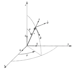
Points in space can also be described by the spherical coordinate system defined in Figure 1.2. The spherical coordinates of r are denoted by (r; (); ¢), where semi colons i

11-side parenthesis always delimit spherical ordinates [Bates and McDonnell, 1989. Sec.

6j.

The spherical ordinates are related to Cartesian ordinates by

x r sin () cos ¢

y r sin (} sin <t> ( 1.8) z r cos ()

The notation can be extended to describe the spatial variation of, say E, in the following different ways: E(r)

=

E(x,y,z)

=

E(r;e;¢).

(20)

z

y

x

Figure 1.2 Graphical representation of the spherical coordinate system in relation to the Cartesian

coordi na te system.

1.1.2 Maxwell's equations

Equations describing electromagnetic waves were formulated by Maxwell [1865]. The time harmonic versions of hIS equations are

[d.

Rudge et al., 1982, p. 7; Jordan and Dalmain, 1968, Chap. 4]

xE

Jm

\7xH

(0"

+

+J

( 1.9) J.t\7·H

_Pm

,,\7·E

₌

_P

where E and H are the electric field and magnetic field respectively, and J the electric current denshy,

J

_m

a fictitious magnetic current density, P

=

the electric charge density,

Pm

a fictitious magnetic charge density,

(J _{the conductivity of the medium,}

[image:20.595.137.440.90.380.2]

(21)

1.1 ELECTROMAGNETIC WAVES

:::: _{the magnetic permeability of the medium,}

\7 the vector differential operator

o. o.

O.

- x + - y + - z

ox

oy

oz

The quantities J and P are considered to be the sources of the electromagnetic wave. The magnetic sources J m and Pm are ficti tious quantities which are often mathem at-ically convenient to invoke (as in, for example, Sec. 2.1.3.1), although from a strictly factual, physical point of view, it is necessary to set _{J m}= Pm = O. The sources vary spatially and time harmonically.

The quantities a, (and tt, are called the constitutive pammetersof the medium and are functions of spatial position. In general they can also be functions of time, but in the time harmonic formulation (1.9) they are assumed to be temporally constant. The constitutive parameters often vary with angular frequency, which in

(1.9)

is represented by w.

1.1.3 Types of llledia

A medium is homogeneous if the constitutive parameters are constant throughout it. An isotropic medium is one in which the constitutive parameters are scalars (implying that they do not depend on the direction of the electric and magnetic fields).

A linear medium is one in which the constitutive parameters do not vary with inten-si ty of the electric and magnetic fields. In a li near medi urn the principle of superpointen-sition holds. This states that if a source distribution produces electric and magnetic fields (EI' Hl ), and another source distribution produces (E2 • H2 ), then when the two source

distributions are applied together, the resultant fields are (El

+

E2 , Hl

+

H2 ).

A good dielectric is a good insulator, implying that a

<t:

WE (compare with the

term in braces in the second equation of (1.9)). A perfect dielectric is non-conducting, implying that a

=

O. A lossless medium is a perfect dielectric in which both E and JL

are real (that is, have no imaginary part).

Free space is a vacuum and is therefore a linear, homogeneous, isotropic. pl!rfect dielectric containing no sources. Free space has a permeability, denoted by Jlv, defined to be 411" X 10-7 henry/metre, and a permittivity, denoted by Ev , which is very close to

(1/3611") X 10-9 _farad/metre.

A good condudor is a medium in which a :?> WE, while for a perfect condudor'

a

=

00. From the second equation of (1.9) it can be seen that, for \7xH and J finite,

E must tend to zero as a tends to infinity. The first equation of (1.9) shows that H tends to zero as E tends to zero (since Jm

=

0). Therefore, an electromagnetic field

cannot exist inside a perfect conductor.

1.1.4

Boundary conditions

Equations (1.9) are the derivative form of Maxwell's equations and are only applicable within a continuous medium. To express the behaviour of an electromagnetic wave at points of discontinui ty of any of the consti t u tive parameters, the integral form of Maxwell's equations [Jordan and Balmain, 1968, Sec. 4.04] can be applied.

(22)

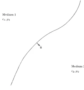
Medium 1

Medium 2

/

Figure 1.3 A surface forming the boundary between two media.

contiguous points on either side of the boundary. Application of the integral equations at the boundary surface yields boundary conditions [Silver, 1949, Sec. 3.3]

fix

Ed

-Jrns

n·

£1 ) _Ps

( 1.11)

fi X (H2 - Hd Js

n·

(/L2H2 /LIHI ) Pms

where

n

is the unit normal to the surface, pointing from medium 1 to medium 2. The terms on the right hand side of (1.11) are called surface currents and surface charges and are distributed over the boundary surface. They are differentiated from the volume sources of (1.9) by the subscript's'.

An important situation arises when one of the media, say medium 1, is a perfect conductor. As pointed out in Section 1.1.3, both and are identically zero, so that (1.11) simplifies to

fix = 0

it·

=

Ps fix

(1.12)

[image:22.595.128.405.70.367.2]

(23)

1.1 ELECTROMAGNETIC WAVES 7

1.1.5 Wave equations

An electromagnetic wave is fully characterized by either its electric field E or its mag-netic field H. By convention, and throughout this thesis, E is usually invoked. From it, one can always calculate H (provided the properties of the medium are known) by rearranging the first equation of (1.9):

H= LYXE

WJ.l (1.13)

For a homogeneous, linear medium containing sources, Maxwell's equations (1.9) can be transformed into wave equations (also called vector Helmholtz equations [Sil-ver, 1949, Sec. 3.6]):

j W J.lJ

+

\7 X J rn

+

~

V' P

E

jwdrn - VxJ

+

..!:.. V' Pm

J.l

(1.1~)

w here I

= [( -

jw J.l)( a

+

jWE )]1/2 is called the propagation constant. For lossless media, it is real and equals the wave number [Ramo et al., 1965, p. 326]:

(l.15 )

where ,\ is the wavelength of the wave. The speed of propagation of the wave is v = W / "

For free space, the speed of propagation reduces to c = (fLyEy)-1/2 which is close to

3x 108 _{metres/second. The index of refroctionof any medium is defined as n}₌_c/v._The

attenuation suffered by a wave as it propagates through a lossy medium is determined by the imaginary part of I [Jordan and Balmain, 1968, p. 126]. In a source free medium, all the terms on the right hand sides of (1.14) are zero.

The Complex Poynting vector P is defined by [ITT, 1968, p. 43-3]

P

=

~(E

X HO) (l.1e; )

It follows from }';laxwell's equations and the law of conservation of energy, that the integral of the normal component of

P.

over the surface enclosing any volume, is the total power flowing out of that volume. Poynting's theorem states that, at each point in space, P gives the magnitude and direction of the average power flow (i.e. power per unit area) [Jordan and Balmain, 1968, Chap. 6].

A my is a curve through space, such that at each point along its length, it is parallel to P [Silver, 1949, p. 110]. A pencil of rays is a thin bent rod shaped volume, of variable cross-section, surrounding a central ray and bounded by a family of rays lying on its surface. From energy conservation principles [Born and Wolf, 1970, p. 115], the total power flow through any cross-section of a given pencil is constant in a lossless medium. Therefore, the intensity of a field along a ray is inversely proportional to the cross-sectional area of a surrounding pencil of rays.

1.1.6 Polarization

(24)

as a distance from the point in space. For a fixed frequency, the locus is an ellipse which lies in the polarization plane [IEEE, 1984].

A field is linearly polarized when the minor axis of the ellipse vanishes, implying that the electric field vector is at all times pointing in the same direction. Two special cases of linear polarization are horizontal polarization, in which the electric field vector is parallel to the earth's surface, and lJertical polarization, in which the electric field vector is perpendicular to the earth's surface.

A field is circularly polarized when the ellipse degenerates into a circle, implying that the magnitude of the electric field vector is always constant. A field which is nei ther linearly polarized nor circularly polarized is called an eLLiptically polarized field. The sense of polarization is the sense in which the ellipse is traversed by the extremity of the real part of the electric field vector.

The polarization unit vector of a field is defined to be [IEEE, 1984]

A

E

t =

TEl

(1.17)

The polarization unit vector of a field completely describes the polarization of the field. Two polarization unit vectors it and i2 , lying in the polarization plane of a field vector E, are orthogonal if il .

ti

= O. The vector E is completely described by its (orthogonal) vector components El and E2 where (d. (1.2) and (1.5))

and (1.18)

When the Cartesian x and y axes lie in the polarization plane, X and

y

form an orthogonal pair of linearly polarized unit vectors. Another possible pair of orthogonal unit vectors are left and right hand circularly polarized [Rumsey et aI., 1951, part III]:

~

l(A

'A)

lR =

J2

x - J Y , 'lL _ =

J2

1(_ x

+

JY

'A)

(1.19)

Note that there can be no component of E in the direction perpendicular to the polar-ization plane.

For arbitrarily oriented Cartesian axes, a field vector is completely defined by the amplitude and phase of all Cartesian components (cL Sec. 1.1.1). Only the phase and relative amplitude of each component is required to define a field's polarization. The polarization of a field is a function of spatial posi tion.

1.2 ELECTRICAL PROPERTIES OF ANTENNAS

An antenna is defined as "a means of radiating or receiving radio waves" [IEEE, 1984]. As seen from the wave equations (1.14), the sources of electromagnetic radiation are charges and currents, where a current is composed of moving charges. A transmitting

antenna provides suitable conditions for radio frequency electric currents to radiate an electromagnetic wave . .A receiving antenna intercepts a radio wave, which induces electric currents on the antenna.

(25)

1.2 ELECTRICAL PROPERTIES OF ANTENNAS

1.2.1

Field

regions

The electromagnetic wave radiated from an antenna can be considered to be composed of two fields. The radiating field is that part of the wave which transports energy away from the antenna. The reactive field oscillates energy between the space near to the antenna and the antenna itself. It is useful to divide the space surrounding the antenna into regions which are differentiated by different characteristics of the electromagnetic wave [Rudge et al., 1982, Sec. 1.4].

The reactive near field region is the region close to the antenna, where the reactive field dominates the radiating field. The reactive field decays faster than the radiating field and, for most antennas, the outer limit of the reactive near field region is of the order of a few wavelengths or less.

The far field region is far enough from the antenna that the angular distribution of the field is independent of distance [IEEE, 1979, p. 139]. The wave consists effectively of only the radiating field, which decays with the inverse of distance from the antenna. The far field region is sufficiently distant that the relative contributions to the radiating field from different parts of the antenna are independent of distance. This implies that the antenna can be treated as if it were a point source with directional variations. Although this condition is only exact infinitely far from the antenna, it is adequately approximated at finite distances greater than the following lower bound [Dlake, 1984, p.122]:

2D2

Rtf

=

-.x-

(1. 20)

where Rtf is the accepted minimum far field distance from an antenna whose largest dimension is D. For small antennas, RIJ should be no less than a wavelength. The part of the radiating field which is in the far field region is called the far field.

The radiating near field region occupies the space between the reactive near field region and the far field region. The radiating field dominates the reactive field, but the relative angular distribution of the radiating field depends on distance from the antenna. The radiating near field region is close enough that the size of the antenna is significant, so the relative contributions to the radiating field from different parts of the antenna depend on distance as well as on angle. The part of the radiating field which is in the near field region is called the near field. The radiating near field region does not exist for antennas which are small compared to a wavelength.

1.2.2 Antenna patterns

An antenna pattern is the spatial distribution of a quantity which characterizes the electromagnetic field generated by an antenna [IEEE, 1984]. The quantity is usually determined over the surface of a sphere which is centred on the antenna. A spherical coordinate system (Sec. 1.1.1), whose origin is at the centre of the sphere, is utilized to locate points on the surface. Only the two angular ordinates (B; 9) are required to specify a point on the sphere, since the radius ordinate is constant.

The gain pattern G(B; 9) of a transmitting antenna is

(1.21)

where Pmd is the power radiated per uni t solid angle in direction

(B;

9) and is determi ned

in the far field region. Pin is the total power accepted from the source. The gain defines

(26)

for power losses within the antenna. The peak gain Gmax of an antenna is the maximum

value of its gain pattern. An antenna with a high peak gain is said to be more directional than an antenna with a lower peak gain and the same power losses.

The effective area Ae of a receiving antenna, connected to a matched load, in the direction (0; ¢) is

( ) Poul

Ae 0; ¢ = Po _me(0") _,cp ( 1.22) where Pout is the power delivered to the load and

Pine( 0;

¢) is the power per unit area of an incident wave radiated from a distant source located at angle (0;

<,6).

The received wave is polarized to produce maximum power output from the antenna (see Sec. 2.2.6). The effective area is a measure of how much power can be transferred from an incident wave to the load.

The amplitude pattern of an antenna is the angular distribution of the amplitude, or the relative amplitude, of a vector component of the electric field. The phase pattern of an antenna is the angular distribution of the phase (relative to some reference phase) of a vector component of the electric field. The polarization pattern of an antenna is the angular distribution of the polarization (Sec. 1.1.6) of the electric field.

The radiation pattern of an antenna is the angular distribution of the complex electric field vector. When the radiation pattern is determined in the far field region it can be called the far field pattern. The far field pattern is is completely characterized by the amplitude and phase patterns of all (complex) vector components of the far field, the peak gain and the power fed to the antenna.

1.2.3

Reciprocity

The principle of reciprocity can be invoked to relate the transmitting characteristics of an antenna to its receiving characteristics.

Consider the measurement of the transmitting characteristics of antenna A, taken at an angle 0 (Fig. 1.4(a)). In practice this is done with the aid of a second antenna

B which is sufficiently far from A to avoid multiple interactions. A voltage source connected to the terminals of A produces a current il through the load connected to

the terminals of B.

Now consider the measurement of the receiving characteristics of A, made for the same angle () (Fig. 1.4(b)), by swapping the voltage source and the load, without moving either antenna. The same voltage source (now connected to the terminals of B) produces a load current i2 at A.

The principle of reciprocity says that the

id

i1 is a constant independent of 0, provided that the antenna system is reciprocal [IEEE, 1979, p. 142]. An antenna system with no ferrite or plasma devices, and embedded in a linear isotropic transmission medium, is reciprocal.

Therefore, the directional properties of an antenna which is transmitting are pro-portional to the directional properties of the same antenna when it is receiving. This means that, in practice, the radiation pattern of an antenna can be measured while it is either transmitting or receiving.

It follows from the reciprocity principle that the effective area of an antenna is related to its gain pattern by the relation [Collin and Zucker, 1969a, Sec. 4.4]

(27)

(a)

lb)

1.2 ELECTRICAL PROPERTIES OF ANTENNAS

()

Antenna A

z

Antenna A

/

f /

/

\ Antenna B

\

I

!

\ ,\ntenna B

\

/

11

[image:27.595.76.454.81.684.2]

(28)

1.2.4 Impedance

In practice, an antenna is connected to an electrical circuit. When transmitting, the circuit provides the current to drive the antenna, and when receiving, the circuit acts as an electrical load for the antenna, abstracting the information carried by the radio wave. In either case, the electrical circuit sees the antenna as an impedance, called the

antenna impedance. To transfer maximum power to and from the antenna, the antenna

impedance must be matched to the impedance (seen by the antenna) of the circuit. The imaginary part of the impedance for a transmitting antenna is due to the re-active energy which is stored in the rere-active field of the antenna. The real part of the antenna resistance is made up of a loss resistance

Rl

oBB in series with the

mdia-tion resistance Rrad. The loss resistance manifests ohmic and dissipative losses in the

antenna. The radiation resistance has a value equal to that of the equivalent resistor which would dissipate the same amount of power that the antenna radiates, if it was connected to the circuit in place of the antenna.

The mdiation efficiency Tlrad of an antenna is the ratio of the power radiated by

the antenna to the total input power [Rudge et al., 1982, Sec. 1.6]. Because the power

dissipation in each of two resistors in series is proportional to the respective values of these resistors, it follows that

Rrad

Tlrad

=

---,-(Rloss

+

Rrad)

(1.24 )

Thus an antenna is efficient if the radiation resistance is much greater than the loss resistance.

1.2.5 Frequency of operation

The antenna performance parameters described so far are defined for a given fixed frequency. However antennas must usually operate over a range of frequencies.

The bandwidth of an antenna is defined as the frequency range over which the

antenna meets all of its specifications. The bandwidth is often expressed as a fraction of the centre frequency, which is midway between the extremities of the bandwidth.

1.2.6 Noise temperature

The minimum signal power that a receiving circuit can detect is limited by noise, which is passed to the circuit from the antenna, and generated by the circuit itself. The noise power N, appearing at the antenna's terminals, is produced thermally within the antenna structure and comes from electromagnetic noise sources in the antenna's environment.

The antenna noise temperatureTA, is the temperature required to cause a resistor to

generate a thermal noise equal to N [Collin and Zucker, 1969a, Sec. 4.8]. Temperature

T, is related to thermal noise power by Nyquist's jormula

N = kTf:J.j (1.25)

where k is Boltzmann's constant and f:J.j is the bandwidth of the system.

(29)

1.3 TYPES OF ANTENNA 13

(1.25), the noise distribution can be replaced by a br'ightness tempemture distribution

Tb(l;l; ¢), such that, for a lossless antenna, the antenna temperature is given by [Rusch and Potter, 1970, Sec. 153]

(1.26 ) In this formulation, Tb(l}; ¢) depends only on the noise sources and is independent of the directional characteristics of the antenna. If the antenna is not lossless, the thermal noise associated with Rlos" also contributes to the antenna noise temperature [Jordan

and Balrnain, 1968, p. 416].

The brightness temperature of an object is equal to its ambient temperature To only if it is a black body, implying that it absorbs all radiation incident upon it. If it absorbs a fraction 0' of the radiation power incident upon it, its brightness temperature

is O'To [Collin and Zucker, 1969a, p. 119]. Non-thermal noise sources usually have a brightness temperature greater than To.

1.3 TYPES OF ANTENNA

There are as many different antennas as there are ways to radiate or receive an elec-tromagnetic wave. Different antennas are suited for operation at different frequencies, have different directional characteristics and have different impedances. Antennas can be loosely categorized into four groups with different modes of operation: current ele-ments, travelling wave, arrays and apertures [Rudge et al., 1982, p. 2]. In this section the salient characteristics and method of analysis of each of these groups is briefly described.

1.3.1 Current elements

Cur'rent element antennas are less than a wavelength in size and are employed for radio frequencies up to about 1 GHz (that is, for )., greater than about 0.3

m).

The simplest radiating source is the elemental dipole (also called the Hertzian dipole or electric current element), which can be physically represented by a short. thin wire carrying a uniform current distribution. From Maxwell's equations, a current I in an elemental dipole of length dl, centred on the origin of a spherical coordinate system (Fig. 1.2) and parallel to the

z

direction, produces a far field pattern of [Collin and Zucker, Hl69a, Sec. 2.2]

607r I dl . /A • E(B;¢)=j e-J21rr _sinBO

).,r ( 1.27)

A shor·t element antenna is one whose length does not exceed about ),,/10 and whose current distribution is approximately uniform. To calculate the radiation pattern of a current carrying wire of any length, one can consider it to be made up of elemental dipoles, and superimpose the contributions of each. For a thin wire with a current distribution of I(z), the far field pattern is [Rudge et al., 1982, p. 52]

E(B;¢)

=

j607rsinB jI(z)e-j2_",r/Adz

iJ

).,r ( 1.28)

The most common type of current element antenna is a half wave dipole, which is a thin wire whose length at mid-band is >./2 and whose current distribution is

(30)

14 CHAPTER] OVERVIEW OF ANTENNA ENGINEERING

dipole, or a loop antenna element, can be constructed from four elemental dipoles con-nected in series, forming a square. A finite sized loop can be considered a distribution (usually circular) of contiguous elemental dipoles. Other derivatives of the elemental dipole include cylindrical rod antennas, vertical radiators and monopoles [Jasik, 1961, Chap. 3].

1.3.2

Travelling wave antennas

The distribution of current on a current element antenna can be treated as the sum of two current waves travelling in opposite directions. A travelling wave antenna is one in which the currents can be represented by one or more waves, usually travelling in the same direction [Walter, 1965, p. 13J. They are typically between 1 and 10 wavelengths long, and operate at frequencies between 1 MHz and 10 GHz. There are two stages to the analysis of these antennas [Rudge et al., 1982, Sec. 1.15]. Firstly, the manner in which the current wave propagates along the length of the antenna must be deduced, and secondly, the contribution of these currents to the radiated electromagnetic wave must be calculated.

One form of travelling wave antenna is a long wire, terminated with a matched impedance at one end, and dri ven at the other. Such an antenna has an approximately uniform current amplitude distribution, with a progressive phase lag [Walter, 1965, Sec. 8.2]. The far field pattern can be calculated using (1.28).

Several terminated long wire antennas can be judiciously oriented and connected, in series and/or in parallel, to reinforce the beams in one particular direction. The rhombic antenna [ITT, 1968, p. 25-9] is based on this principle. In other travelling wave antennas, such as dielectric rod or helical antennas, the wave travels at a speed slower than the speed of electromagnetic radiation in free space [Walter, 1965, Sec. 8.3J.

1.3,3 Aperture antennas

In an aperture antenna the radiated electromagnetic fields can be considered to emanate from a physical opening called an aperture [Collin and Zucker. 1969a, Chap. 3]' which can in practice be anywhere up to several thousand wavelengths across. To achieve a manageable size, aperture antennas are usually operated in microwave bands (which have wavelengths of less than about 0.3 m).

Analysis of an aperture antenna tends to differ from the analysis of other types of antenna, because the radiating field is usually considered to be produced by field elements, rather than by elemental dipoles. The aperture plane is a plane through which most of the radiation passes and is near to, or coincident with, the aperture [IEEE, 1984]. The radiation pattern is computed as the sum of the individual radiations from all field elements in the aperture plane. This is discussed in further detail in Chapter 2.

(31)

1.4 RADIO WAVE PROPAGATION OVER THE EARTH l5

1.3.4 Arrays

An array of antennas consists of several individ ual antennas, called elements, positioned

in a geometrical arrangement which is either regular or irregular. Almost any kind of antenna can be used as an array element, but all the element antennas in single array are usually identical, or at least similar [Ma, 1974, p. 1].

The radiation pattern of the array is the sum of contributions from each of the element antennas [Blake, 1984, Sec. 5.1]. The radiating field contribution of an element antenna depends on its position, its radiation pattern, the amplitude and phase of the signal feeding it and the mutual coupling between it and the other element antennas.

A phased array is one in which the the direction of the main beam is scanned by electronically altering the relative phase of the signal fed to each element antenna. In adaptive arrays, both the relative amplitude and the phase of the signal for each element antenna are controlled (often by computer), to produce a desired time varying radiation pattern [Rudge et al., 1982, Sec. 1.13].

1.4 RADIO WAVE PROPAGATION OVER THE EARTH

Analysis of the propagation of electromagnetic waves between two antennas is straight-forward when they are are within, and far (in comparison to the distance between the antennas) from the edges of, a volume of free space. The transmitting antenna radiates an electromagnetic wave which can be detected by the receiving antenna. Rays from one antenna to the other are straight because the refractive index is constant through-out the volume. The power per unit area of the wave at the receiving antenna depends on the transmitted power and gain pattern of the transmitting antenna and on the distance between the two antennas.

On a dry, still day, when two antennas are close to each other, compared to the distance to the earth's surface and other obstacles, the earth's atmosphere behaves approximately like free space [David and Voge, 1969, Sec. 4.2J. However, the analy-sis of radio wave propagation over or through the earth is usually complicated by the nature of the transmission media involved [David and Voge, 1969; Picquenard. Hl74]. Rays between the antennas can be reflected or refracted due to inhomogeneities in the atmosphere. The power at the receiving antenna can be reduced because of absorp-tion or path obstrucabsorp-tion. These effects vary irregularly with time and depend on the geographical location of the antennas. Some of the atmosphere's effects on radio wave propagation are illustrated in Figure 1.5 and are discussed in the following sections.

1.4.1 The terrain

The earth and sea have conductivities and dielectric constants which are considerably different from those of the air immediately above, and which vary from place to place over the earth's surface [David and Voge, 1969, Sec. 2.2].

When the transmitting and receiving antennas are both near the earth's surface, the part of a radio wave which propagates parallel, and close (at a height of less than a wavelength), to the earth's surface is called a surface wave. Acting in a similar way to

(32)

--

---

--iono' ph",

I

-t...

-

---

--/

- - - -

--

_{troposphere I}

i

I

direc!. wave

I

I reflected wave

(33)

1.4 RADIO WAVE PROPAGATION OVER THE EARTH 17

The earth's surface can also act as a reflector. The part of an electromagnetic wave which is reflected by the ground is called a ground reflected wave and suffers attenuation and a phase shift dependent on the local properties of the terrain [Picquenard, 1974, Sec. 4.1].

1.4.2 The troposphere

The troposphere is the part of the earth's atmosphere in which the average temperature decreases with altitude, clouds form and convection is active [IEEE, 1984]. It is the layer up to about 10 km above the earth's surface. Its refractive index, which is always close to unity, varies randomly with position and time, about a mean which is related to altitude. A standard atmosphere has a refractive index gradient, with altitude, of -0.039 X 10-6 _{per metre [Picquenard, 1974, Sec. 2.1.1].}

The parts of a radio wave which are radiated obliquely into a standard atmosphere undergo progressive refraction and its rays curve downwards, causing it to follow the curvature of the earth to an extent. This means that the direct wave between a trans-mitting and a receiving antenna usually follows a curved path. The length and shape of the path changes due to the slow temporal variations in atmospheric condi tions.

The curved rays, associated with a direct wave propagating through the troposphere, can be geometrically transformed to produce straight rays above a model earth with an

equivalent earth radius, implying an equivalent wave propagating through free space. For a standard atmosphere, the equivalent earth radius is approximately equal to 4/3 of the radius of the earth [Picquenard, 1974, Sec. 2.1.3.2].

Atmospheric conditions are occasionally such that the variation of refractive index with height causes a duct [Hall, 1979, Sec. 2.5], in which the rays are refracted around the earth, thus extending the range of the direct wave to over the horizon. This can only be sustained in a still atmosphere.

Tropospheric scattering is a form of wave propagation attributed to scattering from random irregularities in the index of refraction. These irregularities are caused by turbulence in the atmosphere [Panter, 1972, p. 2]. Tropospheric scattering occurs for frequencies between 0.1 and 10 GHz and considerably attenuates the field. The intensity of the scattered field has a slow seasonal variation superimposed on fast fluctuations having periods of as low as 0.1 second [Panter, 1972, Sec. 12.3.1].

Water vapour and oxygen in the troposphere absorb microwave energy, with the attenuation peaking at about 22 and 200 GHz for water, and 60 and 120 GUz for oxygen [David and Voge, 1969, Sec. 5.4]. The attenuation changes with frequency and with the density of water or oxygen over the propagation path. Particles, especially water droplets, in the atmosphere cause radio wave scattering. For frequencies below 50 GHz, this can produce higher attenuation than that from absorption [Hall, 1979, Sec. 3.4]. The attenuation due to scattering increases with frequency and with rainfall rate.

1.4.3 The ionosphere

(34)

The layers of charged particles are conductive at frequencies lower than about 500 kHz, so waves of these frequencies are reflected by the ionosphere [Picquenard, 1974, Sec. 6.2.1]. Waves with a frequency of between 1.5 and 30 MHz penetrate into the ion-ized layers by several wavelengths and are progressively refracted in a manner which can be equivalent to a reflection. Waves which are reflected or refracted by the iono-sphere are called sky waves, and can be propagated well over the horizon [David and Voge, 1969, Sec. 6.2.3].

Radio waves with frequencies higher than 100 MHz can pass through the ionosphere. The presence of the earth's magnetic field in the ionized region causes the direction of polarization, of a traversing linearly polarized wave, to be rotated: an effect called

Faraday rotation [Picquenard, 1974, Sec. 5.4]. The ionosphere can also absorb an

appreciable fraction of the wave's power.

1,404 Interference

When two or more waves (for example, a direct wave and a ground reflected wave) arrive at a receiving antenna, they form an interference pattern because of their differing path lengths and phase delays [ITT, 1968, p. 21-10J. Therefore, the received power per unit area depends on the receiving antenna position and on the atmospheric conditions at the time. The interference effects can be reduced if the radiation pattern of either the transmitting antenna or the receiving antenna is directional enough to discriminate between the different waves.

There are several sources of electromagnetic noise which can interfere, at the re-ceiving antenna, with the transmitted wave. Atmospherics originate from storms or electrical discharges between clouds, and have a brightness temperature ranging from about 1015 K at 100 kHz to about 100 K at 2 MHz [Jordan and Balmain, 1968, p. 413J.

Artificial noise is produced by electrical equipment, and can have a relatively high level

near towns and cities. Artificial noise power levels decrease with increasing frequency [ITT, 1968, p. 27-4J. Extraterrestrial noise comes from the sun and other stars, and is due to thermal radiation. Cosmic noise varies from about 105 _{K at 30 MHz to about}

1 K at 1 GHz [Jordan and Balrnain, 1968, p. 415J. Particles in the atmosphere which absorb radio wave energy are also a source of thermal noise radiation (cf. Sec. 1.2.6). At the peak absorption frequencies of water vapour and oxygen (see the last paragraph in Sec. 1.4.2), the brightness temperature can be between 20 and 290 K [Hall, 1979, p. 77; Jordan and Balmain, 1968, p. 415].

1.5

SUMMARY

Radio waves are a subset of electromagnetic waves, which consist of time varying electric and magnetic fields. Maxwell's equations (1.9) relate these fields to each other, to electromagnetic sources (time varying currents and charges) and to the constitutive parameters of the media in which the waves exist. The propagating wave nature of radio waves can be demonstrated by rearranging Maxwell's equations to form the wave equations (1.14). A radio wave can be completely described by the amplitude and phase of each vector component of the electric field at each point in space.

(35)

1.5 SUMMARY 19

parameters of an antenna at a given frequency are its radiation pattern, impedance, radiation efficiency and noise temperature (which depends on the environment in which the antenna is operating).

Propagation of radio waves in the vicinity of the earth is affected by the atmosphere and the terrain. The waves can be reflected from the surface of the earth and from the ionosphere. They can be refracted by the troposphere and the ionosphere, and diffracted around the surface of the earth. Particles in the air can absorb and scatter energy from a traversing radio wave. Most of these effects vary, in an irregular manner, with time and with geographical location.

Perhaps the main application of antennas is for communication systems. An oscil-lating current used to drive a transmitting antenna radiates an electromagnetic wave which in turn induces, on a receiving antenna, an oscillating current of the same fre-quency, and proportional amplitude and phase. It follows that any variations in the transmitting current produces proportional variations in the receiving current.

By

en-coding information into these variations, the information can be communicated as the modulation of the radio wave.

(36)

(37)

CHAPTER 2 HIGH GAIN REFLECTOR ANTENNAS

A reflector antenna consists of a feed and one or more reflectors. The feed is a small antenna (or an array of small antennas) which, on transmission, acts as the source of an electromagnetic wave. The reflectors are fabricated from highly conductive mate-rials, so that electromagnetic waves incident upon them are reflected with minimum energy loss. The feed is designed (or chosen) to direct most of its electromagnetic power towards the reflectors. The reflectors are designed (i .e. shaped) to redirect the elec-tromagnetic power in predominantly one direction, thus producing a highly directive radiation pattern.

Section 2.1 outlines approximate methods for analysing reflector antennas, and so provides an understanding of the way in which reflectors affect electromagnetic waves. The performance of a high gain antenna is strongly influenced by its gain pattern, which is discussed in Section 2.2. Different configurations of reflector antennas and their relative merits are discussed in Section 2.3, and in Section 2.4 some applications for high gain antennas are mentioned.

2.1 ANALYSIS OF SCATTERING FROM REFLECTORS

Assume that the source field Eo, from a feed which is far from any other body, is known, either from direct measurement, or from theoretical analysis. When a conducting body is placed in the vicinity of the feed, surface currents J, are induced on the body and radiate a scatteredfieldEs • The total field is equal to [Eo+Esl [James, 1986, Sec. 2.4.1]. The problem of analysing scattering from reflectors is to calculate the total field, gi ven Eo and the shape of the conducting body.

Exact descriptions of scattering from reflectors can in principle be deduced from Ma.xwell's equations (Sec. 1.1.2). However, because these tend to be unmanageable in practice [James, 1986, Sec. 2.4.1], one is usually forced to resort to approximate ap-proaches. The following sections summarize ray optics (Sec. 2.1.1), current-integration (Sec. 2.1.2) and field integration (Sec. 2.1.3), which are all methods of analysing reflec-tor antennas in ways that are inexact but are nevertheless very useful.

2.1,1 Ray optical methods

Classical geometrical optics is that branch of optics which corresponds to the limiting case of k ~ 00 [Born and Wolf, 1970, Sec. 3.1], in which the energy of a light wave