A thesis presented for the degree of
Doctor of Philosophy
in Electrical Engineering
at the
University of Canterbury,
Christchurch, New Zealand
by
Dolf de Roos, B.E. (hans) ~
ABSTRACT
Sonar target classification based on frequency-domain echo analysis is investigated. Conventional pulsed sonars are compared with continuous transmission frequency modulated (CTFM) sonars, and differences relating to target classification are discussed. A practical technique is introduced which eliminates the blind time inherent in CTFM technology.
The value and implications of modelling underwater sonars in air are discussed and illustrated. The relati ve merits of auditory, visual and computer analysis of echoes are examined, and the effects of using two or more analysis methods simultaneously are investigated.
Var ious stat i sti cal techni ques for detect i ng and classifying targets are explored. It is seen that with present hardware limitations, a two-stage echo analysis approach offers the most efficient means of target classification.
A novel design for three-section quarter-wavelength transducers is presented and evaluated. Their inherently flat frequency response makes these transducers well suited to broadband applications.
The design philosophy and construction details of a Diver's Sonar and an underwater Classification Sonar are given. Sea trials reveal that using the Diver's Sonar, a blind-folded diver can successfully navigate in an unknown environment, and locate and classify targets; using the Classification Sonar, targets may be located and classif ied using ei ther operators or computer software.
ACKNOWLEDGEMENTS
Firstly, I must thank my supervisor, Professor Leslie Kay, whose ideas and hypotheses sparked off my interest in this proJect. His intuiti ve grasp on the whole sonar field is extremely comprehensi ve and reflects the lifetime of dedication he has given it.
Professor Kay's propensity to extensive travel abroad has, however, resulted in a large part of my day to day contact being with my associate supervi sor, Dr Peter Gough. Wi th an uncompromising atti tude towards relevance, Dr Gough has provided me with much-valued support and guidance.
Much of the experimental work and system development reported in this thesis could not have been carried out without the skills and enthusiasm of many indi viduals. Thanks are due to Art Vernon, the craftsman behind the di vert s sonar transducers, who never complained about being given yet another des i gn . Together we spent days on end in a shack known as the fish hut, testing a long succession of new transducer deSigns, and later calibrating and matching transducer elements and arrays.
I am particularly appreciative of the contri butions of Mike Cusdin who designed and developed much of the sonar electronics referred to in this thesis. Mike's fifteen years of practical experience in building CTFM sonars is reflected in his engineering proficiency.
system used in the Classification Sonar.
Financial support during various phases of the research is acknowledged from the N. Z. Ministry of Agriculture and Fisheries, and from Edo Western Corporation (Salt Lake City, Utah).
PUBLICATIONS
During the course of the research leading to this dissertation, the following papers were publ ished:
de Roos, A., Kay, L., Cusdin, M.J. & Vernon, A.N. (1981). "A Sonar Aid f'or Divers using Binaural Displays", Ultrasonics International '81 Conference Proceedings, IPC Science and Technology Press, pp 171-175.
Kay, L., Kay, N., Sinton, J.J., de Roos, A. (1981). "Characterization of' Surface and Volume Structure using an Air SOnar with Auditory Display f'or the Blind", Ultrasonics International '81 Conference Proceedings, IPC Science and Technology Press, pp 38-42.
de Roos, Dolf, Cusdin, M.J., Kay, L. (1983). "A Diver's Sonar with Auditory Display", Transactions of the Institution of Professional Engineers of New Zealand, Vol. 10, No.2, July. pp 55-58.
Gough, P.T., de Roos, A., Cusdin, M.J. (1984). "A Continuous Transmission F .. K.. Sonar wi th One Octave Bandwi th and No Blind Time", Proc. 1. E. E. , Vol. 131, No.3. Part F (Special Issue on Sonar Systems). June. pp 270-274.
Cusdin. Michael J. & de Roos, Adolf (1984). "CTFM Sonar Enhances Diver's Eyes wi th Sound", Sea Technology. Vol. 25. No.9, Sept., pp 44-46.
Cusdin. M.J., de Roos, A., Gough, P.T. & Sinton. J.J. (1984). "A Hew Type of CTFM sonar with no Blind Time and a One Octave Bandwidth", New Zealand National Electronics Conference Proceedings, Vol. 21, pp 59-64.
CHAPTER 1
1.1
CHAPTER 2
Abstract
Stack Plot Images Acknowledgements Publications Contents
DfrRODUCTION
THESIS ORGANISATION
CONTENTS
THE CTFM SONAR SYSTEM
i 11 iii
v vi
2
2.1 INTRODUCTION 4
2.2 COMPARISON BETWEEN PULSED AND CTFM SYSTEMS 6
2.2.1 Operating Principles 6
2.2.2 Transducer And Peak Power Constraints 12
2.2.3 Transducer Beamwidth Considerations 13
2.2.4 Range Ambiguities 13
2.2.5 Maximum Range Attainable 14
2.2.6 Trade-off Between Range Resolution
&
Response Time 15 2.2.7 Target Classification Using Continuous Outputs 152.2.8 Ambiguity Diagrams 17
2.2.9 Immunity From Interference 17
2.2.10 Auditory Displays 18
2.3 SUMMARY 20
CHAPTER 3 DUAL DEMODULATION
3. 1 INTRODUCTION 21
3.2 DUAL DEMODULATION 26
3.2.1 Range Ambiguities 27
3.3 PRACTICAL EXAMPLES 27
CHAPTER
4
AIR KlDELLING4.1
INTRODUCTION4.2
SYSTEM ADAPTATIONS FOR AIR OPERATION4.3
EXPERIMENTAL AIR MODELS4.3.1
Fish School Classification4.3.2
Rough Versus Smooth Characterizations4.4
CONCLUSIONSCHAPTER 5
5. 1
5.2
5.3
VISUAL. AUDITORY AND COMPUTER TARGET RECOGNITION
INTRODUCTION SENSORY ANALYSIS COMPUTER RECOGNITION
5.4
EXPERIMENTAL COMPARISONS BETWEEN VISUAL AND AUDITORY DISPLAYS32
33
37 3738
40
41
41
45
46
5.4.1
Auditory Versus Visual Classification Of Fish Models46
5.4.2
Auditory, Visual&
Computer Rough/Smooth Classification48
5.5
CONCLUSIONS51
CHAPTER 6 ECHO PROCESSING FOR TARGET CHARACTERIZATION
6. 1
INTRODUCTION52
6.2
DETECTION STRATEGIES53
6.2.1
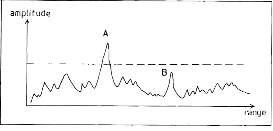
Peak Detection56
6.2.2
Hole Detection59
6.2.3
Maximum Likelihood Detection62
6.3
CLASSIFICATION STRATEGIES64
6.3.1
High Range Resolution Analysis65
6.3.2
Frequency Response Analysis68
CHAPTER 7
DIVER'S SONAR FOR TARGET RECOGNITION
7.1
INTRODUCTION
7.2
TRANSDUCER ELEMENT DESIGN
7.2.1
Adhesi ve Construction
7.2.2
Bolt Construction
7.2.3
Array Configuration
7.3
SIGNAL PROCESSING
7.4
PHYSICAL CONSTRUCTION
7.5
TRIALS
7.6
DISCUSSION
CHAPTER 8
CLASSIFICATION SONAR
8.1
INTRODUCTION
8.2
SPECIFICATIONS AND THEORETICAL PERFORMANCE
8.3
ELECTRONIC DESIGN
8.3.1
The CTFM Sonar Front-end
8.3.2
Spectrum Analyzer
8.3.3
Computer
8.3.4
Displays
8.4
CONSTRUCTION
8.5
OPERATOR CONTROLS
8.6
CONCLUSIONS
CHAPTER 9
DETECTION AND CLASSIFICATION SOFTWARE
9.
1
INTRODUCTION
9.2
EVALUATING SOFTWARE PERFORMANCE
9.3
DETECTION ROUTINES
9.3.1
Local Dominance Of A Peak
9.3.2
Hole Detection
9.4
CLASSIFICATION ROUTINES
9.4.1
Primary
& Secondary Peak Dominance Over Average
9.4.2
Threshold Transgressions
9.4.3
Mean Versus Median
9.4.4
Multiple Invocations
9.5 9.6 9.7
CHAPTER 10
10. 1 10.2 10.2.1 10.2.2 10.3 10.3. 1 10.3.2 10.3.3 10.3.4 10.3.5 10.3.6 10.3.7 10.3.8 10.3.9 10.3.10 10.3.11 10.4
CHAPTER 11
11. 1 11.2
SERIAL VERSUS PARALLEL OPERATION PROBABILITY MAP
DISCUSSION
POOL AND HARBOUR TRIALS
INTRODUCTION POOL TRIALS
Constant Beamwidth And Frequency Response Crosstalk
HARBOUR TRIALS TIle Environment
Operational Procedure
Backscatter From The Seabed Spheres
Tri-planes Drums
Scuba And Snorkel Divers Unidentified Targets Range Resolution
Automatic Detection And Classification Probability Map
DISCUSSION
CONCLUSIONS
SONAR TECHNOLOGY FUTURE DEVELOPMENTS
APPENDIX I APPENDIX II APPENDIX III
This thesis is concerned with systems and processing methods that have potential for improving the classification of obj ects using ul trasound. Four media are commonly probed by ultrasound: mammalian tissue (principally for medical diagnosis), solids (non-destructive testing), air, and water. The research detailed here is primarily concerned with the latter two. Al though air sonars have been in limited use for some time, their use may soon increase dramatically as sonar systems are incorporated into ro bots. However, at present, the most common use of ultrasonics is with underwater sonars.
Underwater sonars for exploring the sea bed generally operate in the high frequency range of 100-500 kHz and are consequently capable of providing useful information up to a maximum distance of around 400m (Flemming et al., 1982) . They suffer severe limitations because of the physi cal properties of the sea as a propagating medium for sound - the only wave energy which can usefully propagate beyond a few metres. Furthermore, the aperture through which the sea and its boundaries are viewed is limited in practical systems to a few tens of wavelengths. and the bandwidth to a few tens of kilohertz, producing azimuthal and radial resolution elements of the order of 1m by 0.1m depending upon system parameters (Lee, 1979).
identifying objects lying on the seabed. Even classifying them as belonging to a set of objects is difficult for distances much beyond 50m.
In areas where debris can be dumped, as in harbours, the problem of distinguishing between man's deposi ts and naturally occurring objects becom es exceedingly difficult. Nevertheless, for both civilian applications (e.g. salvage operations) and military applications (e.g. mine clearance), i t is highly desirable that a means be found for making such a distinction.
Experiments have shown that the porpoise is capable of distinguishing between small objects at least better than man has so far managed (Busnel & Fish, 1980). This establishes that the physical means exists to an extent that man has not yet been able to exploit. Attempts to determine and emulate the essential features of the porpoise's sonar that enable fine discriminations have so far failed.
While many electronic sonars are based on pulse technology and therefore model the biological sonar of the porpoise, there is another cl ass of sonars based on frequency modulation which more closely models the biological sonar of some species of bats. This thesis compares the two general classes of sonars, and shows how the FM system may be more relevant for target classification. Two sonars are described which have been built to test various hypotheses. The results of sea trials indicate that some progress has been made towards the goal of classification.
1.1 THESIS ORGANISATION
The thesis is divided into two parts. In Chapters 2 to 6, the theoretical aspects of sonar synthesis, echo processing and display interpretation are considered in relation to target classification. Chapters 7 to 10 detail the design, construction, and results of sonar systems built to test hypotheses and assumptions.
desi gn. This is followed by a comparison between pulsed, chirped, and CTFM sonars with respect to operating principles and practical limitations.
In Chapter
3.
a technique is described which eliminates the blind time inherent in traditional CTFM sonars. Named 'dual demodulation', the technique is incorporated in sonars described in subsequent chapters.In Chapter 4, the impl ications of modelling underwater sonars in air are considered, and examples are given of models used to check assumptions and help design sonars described elsewhere in the thesis. Chapter 5 compares vi sual, audi tory and computer detection and classification of targets, and considers the consequences of using several processing methods simultaneously. Chapter 6 details the information required for target classification and studies various methods of processing this information.
In Chapter
7.
a diver's sonar is described which can aid mobility and classify objects. The results of sea trials are presented.Chapter 8 details a side scan sonar built to enable both operator and computer target detection and classification. The software written to provide automated detection and classification is outlined in Chapter
9.
while Chapter 10 presents the results sea trials conducted in a harbour environment.CHAPTER 2
THE CTFM SONAR SYSTEM
2.1 INTRODUCTION
Al though contemporary sonar (and radar) designs are predominantly based on pulsed technology, many other techni ques have at some stage been popular. Early radars, for instance. were based on continuous wave interference (CW), and pulsed radars even encountered much scepticism in the mid 1930s when they were first proposed and tested (Skolnik, 1980).
Early sonars used pulses, but during the 1940s, when the war effort spurred intensi ve sonar research and development, CTFM systems became very popular. Kurie (1946) details eleven advantages of FM sonar systems over 'conventional' systems, some of which have at least partially lost their relevance (e.g. relati ve immuni ty from countermeasures) and others which are still relevant today (e.g. continuous and easily monitorable auditory outputs) •
domai n, and require accurate and linear frequency modulators, and spectrum anal yzers with narrow fractional bandwi dth fil ters (or their equi valents). Adequate components were not generally available, and thus while many innovative ideas were postulated, they could often not be implemented. Consequently. FM sonars lagged behind those based on pulse technology.
Meanwhile, bat echo-location had been independently discovered by Griffin (Pierce & Griffin, 1938) and Dijkgraaf (Dijkgraaf, 1943; 1946). Early investigations of bat sonars did not so much influence engineering designs as justify the concept of a man-portable sonar system (Slaymaker & Meeker, 1948). However, the publication of "Listening in the Dark" (Griffin, 1958a) was followed by increased interest in the echolocating systems of bats, many of which use some form of FM sonar. While initial investigations concentrated on analysing bat sonar systems (e.g. Pye, 1960; Kay, 1962aj Kay & Pickvance, 1963), these studies inevitably led to hypotheses that if man's sonars were based on those of bats, comparable resul ts should be achievable (e.g. Griffin, 1958b; Kay, 1962b). More recent research combines refinements of theories on the operation of bat sonars with the development of sophisticated bi oni c sonars. Such research may infl uence signal synthesis (e.g. Al tes & Titlebaum, 1970; Escudie & Hellion, 1975), signal processing (e.g. Johnson & Ti tlebaum, 1976 j Altes, 1976) or target classification (e.g. Skinner et al.,
1977) .
Lately there has been increased interest in CTFM sonars. Although var i ous devices have been developed at the Uni versi ty of Canterbury over the last 20 years, such as blind aids (e.g. Kay, 1974), heart moni tors (e .g. Kay et al. , 1977) , and fishing sonars (Do, 1977) , CTFM technology is now being used in a number of appl ications such as diving (Ametek, 1978 ; de Roos et. al , 1981 ) , side scanning (Gough et. aI, 1984b) and robotics (Kay, 1985). The CTFM principle has similarly found new applications in radars (e.g. Neininger 1977; Clarricoats, 1977).
The enhanced quali ty of CTFM sonar outputs resul ting from current technology has enabled some of the inherent advantages of CTFM over convent i onal (pul sed) technology to be real j sed. For example, range resolution can be traded for response time, and targets can be observed continuously, two features no pulsed sonar can match. Nonetheless, there are still some disadvantages relative to pulsed sonars.
The remainder of this chapter compares CTFM sonars wi th pulsed sonars in terms of both theoretical capabilities and operational practicalities.
2.2 COMPARISON BETWEEN PULSED AND CTFM SYSTEMS
2.2.1 Operating PrinCiples
There are many kinds of sonar technologies, although the differences are often very subtle. The present di scussion considers three general systems: the short pulse sonar. the chirped linear FM pulse sonar. and the CTFM sonar. It is seen that while the output of the chirped linear FM pulse sonar appears Similar to that of the (short) pulse sonar after demodulation, its demodulation process is functionally equivalent to that of the CTFM sonar.
Short pul se sonars radiate a repeti ti ve trai n of pulsed tone. and measure the time delay between the transmission of a pulse and the detection of an echo to determine the range to a target. For a transmitted signal given by the real part of
set)
e
J "2 f 11" c .rect[ tIT t - 1/2]c
for the period 0
<
t<
T and repeated every T seconds, where f is the operating frequency,c
T is the pulse repetition period, and T is the pulse length,
c
(2.1)
e(t) - As(t - 2R/c)
repeated every T seconds. where A is a constant, and
c is the speed of sound.
(2.2)
The range to the target can be determined frOO! the time delay between the transmitted pulse and the echo. since R - c6t/2. where dt is the time delay.
The recei ved echo is passed through a narrowband filter (one whose bandwidth is small compared to the centre frequency) centred on the modulation frequency. whi ch rej ects the out-of-band noi se and thus improves the si gnal/noi se ratio. However. the range resolution, i.e. the ability to di s ti nguish two targets not well separated in range. is improved by transmi tting as short a pulse as possible. Typically. this pulse may be several tens of wavelengths long. but a lower limit of
8
or 10 wavelengths is often seen as a comprOO!ise between the desire for good range resolution and the ability of the bandpass filter to reject the out-of-band noise.Since the average power radiated is proportional to the pulse length, as the pulse length is decreased to improve range resolution, the average power is decreased. As well, the total noise is now increased since the bandpass fil ter must be wi der to pass the shorter pulse. To increase the average power radiated and yet retain the range resolution capability of a short pulse, the transmitted pulse can be chirped. The chirped pulse is many wavel engths long wi th the ini ti al frequency ei ther higher or lower than the terminal frequency; usually this frequency change is linear.
the transmitted signal is the real part of
112 ]
In this case,
(2.3)
for the period 0
<
t<
T, and repeated every T seconds, where f2 is the initial frequency,For a decreasing frequency/time characteristic, f2
>
f1" Now the recei ved echo from a single target at range R (wi th zero target veloci ty) is a delayed replica of the chirp given bye(t) As(t - 2R/c), (2.4)
for 0
<
t<
T, repeated every T seconds.There are two methods of processing echoes recei ved from chirped sonars: matched f1ltering and correlation processing. Both methods, although considerably different in implementation, are equi valent in that both produce the same maximum possible SIN at their outputs (Wainstein
&
Zubakov, 1962).A matched filter is described by
(2.5)
and h(t) x sCoT - t) (2.6)
where H(w) is the frequency response of the filter. h(t) is its impulse response,
Sew) is the transmitted signal spectrum, S*( w) is its com pI ex conj ugate,
set) is the transmitted signal waveform, and oT is a delay required to realise the filter.
Matched filtering is most commonly implemented using the pulse compression receiver (Ohman, 1960) which has a frequency sensitive delay that retards the ini tial frequency by the length of the chirp while not retarding the terminal frequency at all. The process is intended to compress the chirp into an impulse. The output waveform yet) of the matched filter is given by
yet) x
J~
h(1).e(t-1) d1 (2.7)-~
delayed by 6.T and diminished by a factor k, we obtain
(2.8)
Cook (1960) has shown that for a transmitted signal of unit ampl1 tude and of the form of Equation (2.3), yet) is given by
(2.9)
The envelope of the output pulse is seen to have a sinxlx form and the effective pulse width (measured at the -4 dB points) is l/mT - 1/6.f, where 6.f .. f2 - fl' Also, the peak power of the output pulse is k2T6.f compared with the peak input power which was k2• The pulse canpression filter has thus compressed the recei ved pulse by a factor T6.f and increased its peak power by the same factor.
The correlation receiver (Glisson & Sage, 1970) attempts to determine the cross correlation function of transmitted and received Signals, c (T),
tr given by
(2.10)
Assuming a particular received signal may be represented as before in the form
e(t) - ks(t-6.T) (2.11)
we have
Ctr(T) -
kf~
s(t - 6.T).s(t - T) dt. co(2. 12)
The correlation recei ver may be implemented in at least two distinct ways. The most general approach is to mul ti ply the recei ved signal separately by a number of delayed replicas of the transmi tted waveform and to integrate (low pass filter) the outputs. An alternative and less cumbersome receiver may be used if a substantial overlap exists between transmitted and received signals. Such an overlap occurs i f the length of the chirp is made equal to the pulse repetition period. The method involves the direct multiplication of the transmitted and received signals, and forms the basis of the traditional CTFM system.
If the transmitted signal is the real part of
O!it<T (2.13)
and repeated every t seconds to ± ~, the received echo from a single target at range R is
e(t) - As(t - 2R/c) + As(t + T - 2R/c), O!it<T. (2.1li)
From here. repeti tion every T seconds is assumed. and only the real parts of complex representations should be considered.
Let us now demodulate e(t) by multiplying it with a local oscillator which is a replica of set).
gives
Then low pass f11 tering the resul tant signal
d(t) A
e
-j2~(T - 2R/c)mt•
o ::::
t<
2R/c (2. 15a )A
e
-j2~(2mR/c)t•
2R/c :::: t<
T. (2.15b)D(f) - f - 2mR/c (2.16)
for large T where
D(f)
IT
d(t)e-j2nft dt2R/c
(2.17)
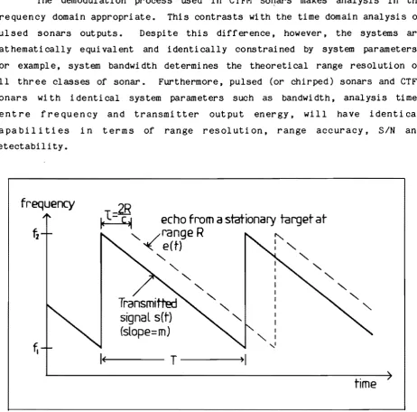
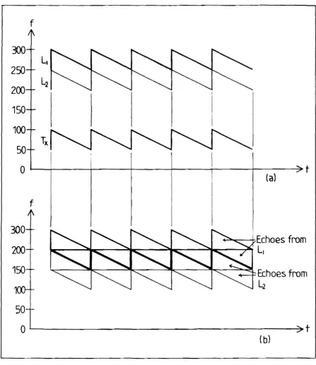
The CTFM system is illustrated in Figure 2.1, which shows a single target at a range R.
The demodulation process used in CTFM sOl}ars makes analysis in the frequency domain appropriate. This contrasts with the time domain analysis of pul sed sonars out puts. Despi te this difference, however, the systems are mathematically equi valent and identically constrained by system parameters. For example, system bandwidth determines the theoretical range resolution of all three classes of sonar. Furthermore, pulsed (or chirped) sonars and CTFM sonars wi th identical system parameters such as bandwidth, analysis time, centre frequency and transmitter output energy, will have identical capabilities in terms of range resolution, range accuracy, SIN and detectability.
frequency
l
-ZH
~ - C ~
echo from a stationary target at
,/range R
I(
~
,
e(t}
,
Transmitted
signal s(t)
(slope=m)
,
, ,
"-
,
T---4
Figure 2.1 CTFM Frequency-Time Characteristic
[image:21.595.62.525.306.762.2]Differences in performance arise because some desired specifications or features may be more readily achieved using one particular system. Thus we are now considering practical limitations rather than theoretical capa biU ties. Many of these differences resul t from the fact that pulsed sonars transmi t energy in a time which is short compared to the pulse repetition period, while CTFM sonars transmit continuously. Some of these differences are discussed in the following sections.
2.2.2 Transducer And Peak Power Constraints
Pulsed and chirped sonars require only one transducer. which is connected to the output of the transmitter power amplifier during pulse transmission. and to the input of the receiver pre-amplifier during reception. However. since CTFM sonars transmi t and recei ve continuously. these sonars requi re two separate transducers. This requirement represents a severe limi tation on CTFM systems in terms of both cost and transducer mounting logistics. Acoustic baffles may also be required to reduce crosstalk between the two transducers.
Since the transmi tter duty cycle of pulsed sonars is small (typically 0.1%). all the radiated energy must be transmi tted during a time which is short compared to the sweep repetition period. and so the peak power tends to be very high. However. the peak power that can be radiated underwater is limited by cavitation. Conversely, since the transmitted duty cycle of CTFM sonars is 100%. the average energy transmitted can be high using only moderate instantaneous power levels with no difficulties caused by cavitation.
2.2.3 Transducer Beamwidth Considerations
Beamwi dth is determined by aperture dimensions and wavelength. The beamwi dth of a pulsed sonar is thus fixed by the si ze of the transducer and the frequency of operation. Furthermore, since pulsed sonars can operate using a single transducer, most (though not all) are operated in this manner, in which case the transmit and receive beamwidths are identical.
However, the operating frequency vari es for CTFM and chirped sonars and the beamwidth changes correspondingly. For a CTFM sonar with a one octave transmi t ted frequency band, the beam wi dths at opposi te ends of the sweep differ by a ratio of 2:1. In some CTFM sonars, such changes in beamwidth are tolerated: these sonars usually have auditory displays, and sweep periods of less than around 250 ms, so that the ear integrates the output (e.g. Kay, 1974; de Roos et al., 1983). I f the changing beamwidth is considered undesirable, methods of reducing the variation must be applied. Some sonars incorporate electronic networks which provide frequency selecti ve shading of the transducer el ements to al ter the effecti ve radiating aperture (e.g. Smi th. 1 972) •
The beamwi dths of a sonar 's transmi tter and recei ver need not be the same. For example, scanning sonars may transmit using a broad beam, and recei ve using a narrow scanning beam to determine the direction to targets (alternatively, a broad-beam receiver may pick up echoes transmitted by a narrow scanni ng transmi tter). Similarly. a side scan sonar using narrow transmitter and receiver beams may suffer from minimal overlap of the transmit and recei ve sectors owing to forward vessel motion. Making ei ther beamwidth broader will increase the likelihood of receiving Signals from the desired sector (at the expense of increased crosstalk and possibly nOise, depending on which beam is broadened).
2.2.4 Range Ambiguities
will then vary, while real targets will always appear in the same positions. Of course, more than one pulse repeti tion period is then required to resolve the ambi gui ti es .
In CTFM sonars, range ambiguities can occur at ranges of lcT/2 + Rand lcT 12 - R, as the system demodulates echoes which are both higher and lower in frequency than the local oscillator signals. With traditional CTFM sonars. the maximum range tends to be much less than cT/2, and the extra transmission loss (due to absorption and spheri cal spreading) to phantom targets ensures that these tar gets are well at tenuated. Chapter 3 introduces a CTFM demodulation system where the maximum range may be a large proportion of cT/2, and considers range ambiguities for these sonars.
2.2.5 Maximum Range Attainable
All acti ve sonars are constrained by the general sonar equation, one form of which is gi ven by
2TL SL - (NL - DI) - DT + TS (2.18)
where TL is the one way transmission loss; SL is the transmitted source 1 evel ; NL is the noise level
DI is the directivity index of the recei ver; DT is the detection threshold; and
TS is the target strength.
2.2.6 Trade-off Between Range Resolution And Response Time
T he range r esol uti on of a pul sed sonar is determi ned by the transmi tted bandwidth, and to a first approximation equals c/AF, where c is the speed of sound and AF is the bandwidth (Benjamin, 1966). Once the bandwidth and maximum range have been fixed, the range resolution and response time are also fixed.
The optimum range resolution attainable with a CTFM sonar is also c/AF (Gough et al., 1984a). However, a feature of any CTFM system is that range resolution is not determined by the form of the transmitted waveform. The outputs of CTFM sonars appear in the frequency domain, and hence must be analyzed using some form of spectrum analysis. Since the response time of a spectrum analyzer is proportional to the bandwi dth of the indi vi dual bandpass filters, by making these filters less selective, they respond more rapidly. Less selective filters also encompass greater radial ranges, so that range resolution can be traded for speed of response. ThUS, the full demodulated output of a CTFM sonar may be covered with a few wideband filters having a rapi d response time, or many narrowband filters having a slow response. For example, the area observed by a sonar may be rapidly and continuously scanned; as soon as a target is detected, it may be examined in much greater detail, albeit less rapidly.
2.2.7 Target Classification USing Continuous Outputs
CTFM sonars, on the other hand, transmi t continuousl y and therefore receive echoes continuously fran all targets. Consider a single target in the field of view of a CTFM sonar. If the target strength (TS) is just sufficient for the obj ect to be detected wi th a si ngl e pul se of a pulsed sonar constrained by the same time-bandwidth product, then the continuous echoes recei ved by a CTFM sonar will be weak, and detection will only occur using a narrow filter wi th a response time of one sweep peri od (Cook & Bernfeld, 1967). However, if the TS is greater than this minimum required for detecti on, then range resol ution can be traded for response time. The target will then be detected after a shorter period, and hence observed more frequently within the same analyzer filter during a single sweep. Furthermore, if the response time of the analyzer filter in use is sufficiently short, and the TS of a target is sufficiently large so that detection is achieved wi thin this filter response time, then observation (auditory or visual) of the target appears continuous.
There are two important benefits of a continuous display which can Significantly improve target classification. Firstly, if a target exhibits characteristi c motion, there are likely to be characteristi c vari ations in echo strength and Doppler shifts. Continuous observation of these echoes may enable target identification. For example, the indi vidual and group motions of fish comprising various schools are often characteristic of their species (Holliday, 1974). The ability to observe this motion (visually or aurally) provides additional information which may lead to school identification. Such identification may be impossible with the 'windowed' output of a pulsed sonar: by Shannon's sampling theorem, a pulsed sonar will only be able to reconstruct repeti ti ve target motion if the period of the motion is less than half the pulse sonar repeti tion peri od. Furthermore, such reconstruction requires the echoes of several pulses; in contrast, the frequency of repeti ti ve target motion detectable with a CTFM sonar is limited by the response time of the analysing filters, which, as was seen above, may be reduced to much less than a sweep period.
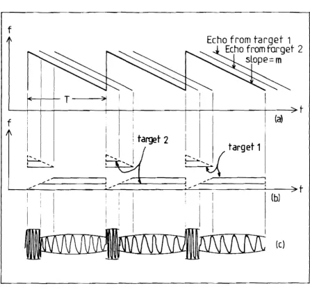
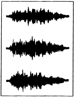
signatures are useful for target classification (Kay et al., 1981) using visual, auditory or electronic analysis. Although echoes from pulsed sonars constrained by the same time-bandwidth product will contain the same total information, this information is more difficult to analyze since it is all contained within a relatively short pulse echo. In comparison, the outputs of CTFM sonars are readily processed to generate 'stack plot displays' or spectrograms (see Figure 1, page 11), whi ch are pseudo 3-dimensional representations of the the frequency signatures of targets. SUch a display is described in Chapter 8 and extensively illustrated in Chapter 10.
2.2.8 AmbIguIty DIagrams
Ambigui ty diagrams are used to establish the ability of various waveforms to resolve range and Doppler uncertainties. The deri vation of ambiguity functions for pulsed systems is well documented (e.g. Woodward, 1964; Skolnik, 1982). An introduction to ambiguity diagrams for linear FM sonars is gi ven by Russo & Bart ber ger (1965). Thi s wor k is extended to wi de bandwidth systems by Kramer (1967), Bates (1971) and Sibul & Titlebaum (1981). A com prehensi ve derivation of ambiguity functions for wideband CTFM sonars is given by Do (1977).
2.2.9 ImmunIty FrOID InterCerence
fact ors whi ch make pul sed sonars more suscepti bl e to thi s ki nd of interference.
Impulsi ve noise frequently comprises wideband energy, sane of which may readily intrude a pulsed sonar's recei verj linear sweeps must not only have energy across the CTFM sonar's operating bandwidth, but they must also sweep at precise rates and in the correct sense. Furthermore, impulsive phenomena are more prevalent in both nature and man-made environments. Consider the appl ication of sonars to robots in an industri al environment. The sources of noise in such an environment are almost exclusively impulsive or of continuous frequency. Under these condi tions, CTFM sonars are less likely to register phantom targets from spurious sources.
2.2.10 AudItory Displays
In contrast to animal sonar systems in which sonar echoes are processed by the audi tory system, the primary displays of electronic sonars (and radars) have nearly always been visual. Audi tory outputs are sanetimes included in systems to provide confirmation of visual displays (Winder, 1975) or improve localization (Scorer & Watkins, 1977), but they are seldom used independently.
Time expansion of the audi tory output can be used to overcome the precedence effect. This expansion may be configured to bri ng the recei ved frequencies directly into the frequency band sui table for human perception. For example, the pulses emi tted by the dolphin tursiops truncatus have been emulated and the received echoes time expanded by a factor of 50 to enable subjects to discriminate various targets (Martin & AU, 1978). However, time expansion is implemented at the expense of real-time analysis: expansion by a factor of 50 results in only 1/50th of all signals received being analysed.
The demodulated outputs of CTFM sonars, on the other hand, are ideally sui ted to audi tory analysis. Mammalian audi tory systems are modelled by a bank of filters (Altes & Reese, 1975; Neuweiler et al., 1980); Hunt (1972) describes narrowband filtering 1n the frequency domain as the signal processing adjunct to the human ear. Kay (1962b) has shown that range es ti mati on is superi or usi ng frequency domai n range coding compared to audi tory estimates of delay using pulsed systems. Furthermore, two closely spaced targets are readily discerned using a CTFM sonar. For example, Roederer (1975) reports that two tones in the neighbourhood of 2,000 Hz must be separated by some 200 Hz to be discriminated. For a typical air sonar with a range code of say 1800Hz/m, this corresponds to a range resolution of around 11mm. Do & Kay (1977) report that a frequency separation of up to 40% is required to discriminate the tones; if the targets are placed closer together, the tones may not be separately di scerni bl e, but the resul tant beat frequency will indicate the presence of the second target. In add1 tion to providing range information, binaural CTFM displays can provide azimuth information, while the precedence effect degrades lateral localization in pulsed systems
(Rowell, 1970).
2.3 SUMMARY
Studies of mammalian sonar systems have influenced electronic sonar des i gns. While pulsed sonars operate in a manner similar to the biological sonars of many marine animals. CT.FM sonars model those of various bats. FM sonar technology has lagged behind pulsed technology largely because adequate components were unavailable; now that most of the CTFM related operations can be adequately implemented electronically. some of the inherent advantages of CTFM sonars can be realised. These advantages may be summarised as follows:
1. Low instantaneous transmitted power levels ease transducer design constraints.
2. CTFM sonars may have a greater energy output which can result in a greater maximum range.
3. Whereas pulsed sonars have windowed outputs. CTFM sonar outputs may be perceived continuously. which can facilitate target classification.
4. Range resolution can be traded for analyzer response time.
5. CTFM sonars may be more immune to interference from typical spurious sources of noise.
6. CTFM outputs may be effectively processed aurally.
Against these advantages the following disadvantages must be noted:
1. Two transducers are required;
CHAPTER 3
DUAL DEMODULATION
3.1 INTRODUCTION
Despite the fact that CTFM sonars transmit and receive continuously, the demodulated output corresponding to a single stationary target is not continuously present as a single frequency. The discontinuity arises because the transmitter must be periodically reset to its initial frequency.
Recall from Section 2.2.1 that the demodulated output of a traditional CTFM sonar for a single target at, range R is given by
d(t) A e -j2n(T - 2R/c)mt ,
o
:$ t<
2R/c <3.1a) Ae- j2n (2mR/c)t 2R/c :;; t<
T. <3.1b)components are unwanted, and the usual procedure is to eliminate them by ampli tude modulating the outputs of the VCO and the receivers in such a way tha t the ampli tude is reduced to zero some time before reset, and increased again, in a controlled manner, some time after. Thus the output is blanked when reset occurs, resulting in a hiatus known as 'blind time' (or sometimes
'lost time').
f
f
I
I
Echo from target 1
Echo from target-
2
sLope= m
H+
T---3i'I
t:.::....:
.
.
...Figure 3.1
I
I
target
1
target 2
I
' ... I
~,-'(
~
~r---~ ,-,~---~
(b)
[image:32.597.68.515.232.659.2]the signal at the sweep repeti tion rate. When analyzed aurally, the echo signal is heard as an interrupted tone, and the quality of this tone is degraded as the proportion of blind time is increased (Kay, 1980). While the modulat ion of the auditory output produced by blanking may be relatively unobtrusi ve wi th sweep repeti tion periods greater than around 200 ms, for shorter range devices (such as children's blind aids), the modulation becomes intrusive, and perception of the sweep rate may mask the desired target sounds (Hodgson
&
Boys, 1977).Secondly, implementing the blanking usually involves using a series of timing circuits and a multiplier. These circuits may require considerable trimming for adequate suppression of the reset induced signal discontinuities.
Thirdly, the proportion of the transmitted sweep which must be blanked will depend on the maximum range at which the sonar has been set to operate, as the blanking must cover both the transmitter flyback and the received echo flyback for targets out to the maximum range. Consequently, for small maximum ranges (1. e. where Rmax is much less than cT 12), blind time is less noticeable than for large maximum ranges (when Rmax becomes a significant portion of cT/2) in which case the sonar may be blind for a large portion of its sweep repetition period. This is one of several reasons why the demodulated bandwidth of practical CTFM sonars has tended to be limited to some 10% of the transmitted bandwidth.
Fourthly, there may be an adverse effect with the sudden application of the signal D(t) to spectrum analyzers. Many analyzers comprise banks of high Q-factor bandpass fi lters which are somewhat underdamped to aChieve max imum selecti vi ty. The sudden application of the signal D( t) may produce unwanted transients in all of the bandpass filters, and these transients can mask a weak signal.
zeros spaced apart by lIT. Furthermore. two targets are considered to be resolved if there is a 3 dB dip between the spectral components corresponding to the targets. Consequently. if the demodulated outputs of two targets are available for an entire sweep period T. the targets will be resolved if they are spaced apart by 2/T. This result is apparent when the two frequencies are centred on spectral lines of the line spacing. but holds true in general. However. as a result of blanking. the demodulated outputs are available for less than an entire sweep period. Recall that blanking is effectively implemented by multiplying the sonar outputs with a rectangular function. In the frequency domain. this multiplication corresponds to a convolution with a si nc function. the effect of which will be to broaden the spacing between the zeros of the sinc function corresponding to the target (Kay. 1980). Consequently. the resolution will be reduced to 2/{T-b). where b corresponds to the length of the blanking pulse.
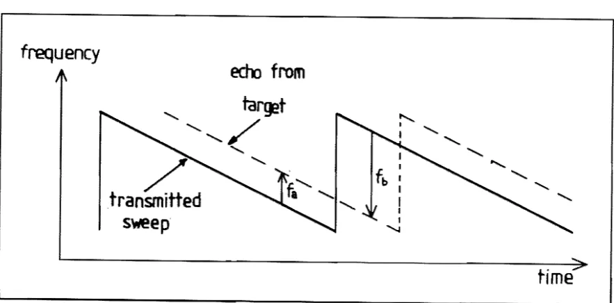
The only previous operational CTFM system wi thout any blind time was the Delta-Cobar sonar developed during the early 1940s (Kurie, 1946). An operator would moni tor the sonar I saudi tory output, which would produce two tones for a target during the sweep, as given by Equations (3.1a) and (3.1b). These tones are shown as having frequencies fa and fb in Figure 3.2. The operator would vary the sweep period T until the auditory output was heard to have a single frequency during the entire sweep. Under these conditions, fa
=
fb in Figure 3.2, and T =4R/c
in Equation (3.1a), where R is the range to the target being examined, thereby equating Equations (3.1a) and (3.1b). The range of the target could then be read off a calibrated sweep period dial. However, as there would only be a continuous and constant frequency for targets in a single range annulus, the exception of the Delta-Cobar system is rather academic.frequency
edlJfrom
ta~t
"
.../
/
transmitted
s~ep
,
,
time
[image:35.595.70.512.390.608.2]3.2
DUAL DEMODULATIONConsider a sonar system using the same transmitted signal set) and the same received signal e(t) as given in equations (2.13) and (2.14). However, instead of demodulating e(t) by s(t), let us use two demodulators with two local oscillators having outputs L1(t) and Lz(t) where
L (t) +j2n(fl + kmT)t -j2nmt
Z
1
=
e .e <3.2)and
L (t) +j2n(f1 + {k-1}mT)t -j2nmt
Z
2. .. e .e
where 0
<
t<
T and k is any integer such that k ~ 2 - (f/mT). I f D1 (t) is the output from the first demodulator and Dz(t) the output from the second demodulator, thenI
A~
e- j2n ( IkimT - Ik-1 12mR/c)t + G(t)i=1
<3.4 )
for all t, where G( t) comprises all signals outside the frequency band I k I mT to Ik-1ImT, and is usually filtered out. Note that there is now no blind time and Rmax is only limited by the sweep repetition period T so that Rmax may extend out to cT/2. Of course, there may be good reasons for limi ting the useful range to much less than cT/2, such as range ambiguities, and spectrum analyzer capabilities.
The demodulated frequency associated wi th zero range is I k I mT, while that associated with the maximum range Rmax == cT/2 is Ik-1ImT. Hence for all
posi ti ve integer values of k, the range will be reversed wi th respect to demodulated frequency, with zero range at a higher frequency than the maximum range. Furthermore, for all values of k other than zero and one, the demodulated output will not be at baseband (DC to +mT). In these situations, the outputs can be brought down to baseband by a third demodulator with a fixed local oscillator at
f == Ik-11mT for k ~ 2 <3. 5a)
Al ternati vely. the spectrum analyzer can cover the demodulated frequency band if this is more convenient.
3.2.1 Range AmbiguitIes
It was shown in Section 2.6 that whereas range ambiguities in pulsed sonars occur at multiples of the maximum range, so that a target displayed as being at a range R may in fact be at tcT/2 + R. where t is an integer. range ambigui ties in traditional CTFM sonars may occur at ranges of tcT/2 + Rand tcT/2 - R. as the system demodulates echoes which are both higher and lower in frequency than the local oscillator signals. Furthermore, recall that in tradi tional CTFM sonars, since the maximum range Rmax tends to be a small portion of cT/2 (to keep the blind time small), the range corresponding to the first ambiguity (cT/2 - R) is much greater than the displayed range R, and the extra transmission loss ensures that the phantom target is well attenuated.
However, in dual demodulation CTFM sonars, where Rmax can be a significant portion of cT/2, the signal strengths of phantom targets can be comparable to those of real targets. I t is possible to eliminate range ambiguities at ranges of cT/2 - R. For example, using narrow bandpass filters. cascaded mixers and single sideband techniques, circuits can be designed to force the system to use only echoes above (or below) the local oscillator. These techniques will reduce the range ambiguities to those of pulsed sonars at the expense of circuit complexity.
3.3 PRACTICAL EXAMPLES
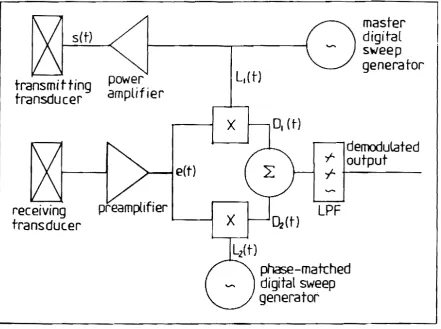
Recent advances in digital frequency synthesis have made interlaced or multiple local oscillator techniques feasible. More specifically, the advent of repeatable, linear and phase-controllable swept frequency generators make the interlaced dual demodulation system described above quite practical.
This transmit sweep also doubles as the first local oscillator Ll , so that k of equations 3.2 and 3.3 is zero. The second local osc illator L2 is synthesized to join onto the end of Ll , and sweeps down from 50 kHz to 25 kHz as shown in Figure 3.3(a). Since Ll(t) is phase matched to L2(t), there is no phase discontinuity at the point where D2 takes over from D1• The recei ved
echoes are demodulated directly to baseband (DC to 25 kHz) as shown in Figure 3.3(b), and the signals are fed to a spectrum analyzer. Rmax has been limited
to 0.5cT/2 in order to reduce range ambiguities.
sonar is shown in Figure 3.4.
A block diagram of this
o
o
f
L-~--~---~---4---r--~---r----~t
Figure 3.3 Dual demodulation system with k
=
0 showing (a) transmitter and local oscillator signals and (b) demodulated signals.(a)
[image:38.600.73.539.259.624.2]transmitting
transducer
[image:39.595.65.507.110.439.2]receiving
transducer
Figure 3.~
eft)
preamplifier
master
digi tal
sweep
LI(t)
generator
X
X
L
2(t)
demodulated
-I-
output
-r
...
LPF
phase-matched
digital sweep
generator
Block diagram of dual demodulation system.
A focussed, high resolution scanning air sonar has also been developed using dual demodulation. As wi th the previous sonar, the parameter k of equations
3.2
and3.3
is zero. but now the transmitter and first local osc illator Ll sweep down from 200 kHz to 100 kHz. while the second local oscillator sweeps down from 100 kHz to DC. Further, the maximum range is made equal to cTf2, as the sonar is intended for use at a robot work station, and it is assumed that there are no objects beyond the maximum range to give rise to phantom targets. (Echoes from objects beyond the maximum range would in any case be relatively weak as a result of being out of the beam's focus.)of a cons lderably higher frequency than the transmi tted sweep, as shown in Figure 3.5(a). One of the reasons for thi s choi ce of k is that the demodulated outputs, shown in Figure 3.5(b), fall outside the transmitted bandwidth, thereby reducing any feedthrough frequency components. This sonar forms the basis of the Classification Sonar described more fully in Chapter 8.
f
?l)()
250
200
150
100
50
0
f
50
L.
~
Tx
t
(a)
...--..;::--t;Echoes from
~----~r---~~~--~~----~E---~~
L,
Echoes from
L2
O~---7t
Figure 3.5
( b)
[image:40.597.61.509.184.701.2]The blind time inherent in traditional CTFM sonars results in ampl1 tude and phase discontinuities which adversely affect audi tory analysis of sonar outputs and electronic spectrum analysis.
degrades range accuracy and resolution.
Furthermore, blind time
CHAPTER .II
AIR MODELLING
4.1 INTRODUCTION
While sonars are most commonly associated with underwater devices, the use of sonars in air goes back a long way - indeed, the first patent relating to sonars was for an air application (Richardson, 1912). However, the advantages of sound as a propagation source over light are much less in air than they are in water. The attenuation of sound, for instance, is two orders of magnitude greater in air than it is in water; conversely, light is barely attenuated in air, but propagates poorly in water. Similarly. while factors reducing aquatic vision (e.g. silt) hardly affect the propagation of sound in water, atmospheric conditions that reduce vision, such as rain, dust and fog, do impair the propagation of sound. This impairment is illustrated by echolocating bats, which turn back on fog as if it were a solid wall (Pye, 1971) . Not surprisingly then, air sonars are most frequently employed where vision is impossible or difficult.
One use of air sonars is as mobili ty aids for the blind or partially sighted (e.g. Kay, 1974). Such devices have been developed at the University of Canterbury for the last 20 years. Early devices consti tuted simple obstacle indicators (Kay, 1964), while recent devices incorporate binaural di splays and prov ide suff i c ien t audi tory information to enable target classification (Kay et al., 1981).
comparatively poor angular resolution, but accurate range resolution. Hence, a combined system using optics for angular resolution and sound for range resolution may be useful. Sonars may also be useful in robotics applications where adequate lighting is difficult to provide, where objects are optically transparent, or where background objects confuse the optical processor (Marsh etal.,198lJ).
There is, however, a further use for air sonars, namely to model underwater sonar systems. Underwater tri als are usually expensive and difficult to control, while air modelling can be versatile, and the cost is usually small compared to the value of information acquired. Much less physical space is required (distances must be scaled down in the model), and trials are not dependant on swimming pool, vessel, or crew availability, harbour board au thor i ty, or favourable weather conditions. However, the literature does not suggest that air sonars are often used for this purpose -most sonar modelling is analyti c or mathematical, rather than physical. Nonetheless, Smith (1972) tested his sonar in air to confirm performance prior to sea trials, while Cram and Staveley (1977) used a scale model air sonar to model radar systems.
This chapter considers some of the factors involved in air modelling, and illustrates these with some practical examples.
~.2 SYSTEM ADAPTATIONS FOR AIR OPERATION
Sound waves are propagated pressure and density fluctuations in the medi urn caused by particle motions.
equation can be expressed as follows:
For small amplitudes, the general wave
o
where p p(x,y,z,t) is the dynamic pressure, c c(x,y,z) is the speed of sound, and
~2 = the Laplacian operator.
The simplest description of the sound field is the solution of the wave equation in one dimension (x) as a sinusoidal plane wave represented by
p(x,t) po.sin( 2~x/A - 2nft + ~ )
where Po is the amplitude of the pressure fluctuations, A is the wavelength,
f is the frequency, and
~ is the phase shift.
This equation can also be expressed as
p (x, t) po.sin( kx - wt + ~ )
where k
=
2~/A is the angular wave number and w = 2nf is the angular frequency.(4.2)
While these relationships apply in air as well as in water, there are some fundamental differences in wave transmission between air and water which are now considered.
The speed of propagation of a physical disturbance in a medium is largely dependant on the density of the medium. Water is considerably more dense than air, and thus the speed of sound in water is much greater than it is in air. Tables are available giving the speed of sound as functions of humidity, temperature, pressure, salinity, etc (e.g. Weast, 1981). For the purposes of the discussion to follow, it is assumed that the speed of sound in air is 300 mis, and that in water it is five times greater, at 1500 m/s.
As a result of this difference in speed, the maximum range attainable so as to avoid primary range ambiguities (cf. section 2.2.4) in air will be one fifth as great as i t is underwater, (for a given sweep period for CTFM sonars, or pulse repetition period for pulsed sonars), all other things being equal. The slower speed of sound in air is one of several factors limiting the maximum range attainable using air models.
spreading is the same underwater as it is in air. and is deri ved by simple geometry to be 6 dB per doubling of distance for a one-way transmission path.
The at tenuation due to absorpti on vari es considerably wi th such f actors as temperature, pressure. and (in water) salini ty. In both air and water, absorption increases dramati cally wi th increasing frequency, and thus the operating frequency severely limits the max imum range at tainable. However, at 80 kHz and 20°C, the absorption of sound in water is typically 0.02 dB/m, while in air under the same conditions it is 2.9 dB/m, or 24 times as great. The absorption of sound in air is the greatest factor restricting the maximum range attainable with air sonars.
The slower speed of propagation and higher absorption of sound in air reduce the maximum range of an air sonar compared to that of the underwater sonar being modelled. In modelling an underwater CTFM sonar in air, the sweep rate is usually increased to achieve a comparable demodulated bandwidth. By maintaining the demodulated bandwidth, it is possible to use the same spectrum analyzer used for the underwater sonar being modelled. However, the shorter sweep period will broaden the line spacing in the analyzer output, and the analyzer must now be able to capture the data in a shorter time.
For any periodic disturbance,
c = H (4.4)
where c is the speed of propagation, A is the wavelength, and
f is the frequency.
Thus for a given frequency of operation, a decrease in speed results corresponding decrease in wavelength. I f a target is encompassed
in a by n by 5n i t is wavelengths underwater, then that same target will be encompassed
wavelengths in air (assuming no change in frequency of operation). If
desired to retain a given number of wavelengths across a target, then for a fixed frequency of operation, the model of the target will have to be scaled down by a factor of five. Alternatively, the centre frequency can be altered, but a choice must then be made between maintaining the original bandwidth or maintaining the proportion of an octave over which the transmitter sweeps. The former is important in scaling range accuracy and reSOlution, and the latter may be necessary to avoid harmonics.
centre frequency may be adjusted simultaneously.
A further factor to be considered in modellIng underwater environments in air is the relative characteristic impedance of targets and the propagating medium. The extent to which some of the incident sound penetrates the target depends on the impedance mismatch between the target and the medium. If there is no mismatch, there wi 11 be no reflection and the target will be acoustically transparent. Conversely, a large mismatch results in most of the incident energy being reflected.
Since the characteristic impedance of air is orders of magnitude less than that of typical targets, most of any incident sound is reflected, and thus received echoes are caused by reflecting pOints on the surface of the target. In water, however, the characteristic impedance of the medium is much closer to that of many typical targets. As a result, there is considerable target penetration by the incident sound, some of which is reflected by discontinui ties wi thin the target (i. e. where there are further boundaries between materials of different characteristic impedance). The reception of echoes from within a target may facilitate the identification of that target. For example, the characteristic impedance of fish flesh is so similar to that of water that the echo from the water-flesh interface is very small. Most of the sonar echo originates from the flesh-air interface created by the swim-bladder, an air-sac used by most species of fish for breathing (Tucker, 1967).
Although background noise and reverberation are generally not modelled in air, they can be considerable in water (espeCially the sea). Hence, resul ts using air models that take no account of background noise or reverberation should be interpreted with due caution.
and furthest ranges, then the maximum range of the air model has to be reduced. Hence, any air model will be a compromise. wi th some parameters being scaled more accurately than others.
Finally. while most of the underwater sonar electronics can be used in the air model if desired. the underwater transducers are totally unsuited for use in air. The most common underwater transducer element is a piezo-electric ceramic, clamped between two sections of material used to modify the characteristics of the element and to improve coupling to the medium. The condenser transducer (Kuhl et al., 1951t) typically used in air comprises a grooved metal back-plate covered wi th a sheet of mylar, the outer layer of which is coated wi th a thin layer of conducti ng material. Since air transducers are completely different to underwater transducers, the transmitter power amplifier and receiver pre-amplifiers must also be replaced.
4.3
EXPERIMENTAL AIR MODELSVarious air models were used to derive results presented elsewhere in this thesis. Some of these are described to illustrate the modelling process.
4.3.1 Fish
School ClassificationState-of-the-art sonars used by fishermen do not prov ide easy recognition of fish species. A recent study reports that 50% of commercial fishermen consider the major problem with their sonars to be a lack of species identification (Kanciruk. 1983). Any success at identifying targets is based largely on sonar operators' familiarity with fishing zones and their knowledge of the habits of species sought, such as school velocity and swimming depth. Hence fishermen would greatly benefit from sonars that could distinguish between different schools of fish. A number of attempts have been made at making such discriminations (e.g. Holliday, 1912. Deuser et al., 1919).
conf igured to sweep from 100kHz to 55kHz in 80ms, gi ving a range code of 3400Hz/m, and a range accuracy of 7.3mm. A binaural receiver was used with the two receiver transducers splayed 15 degrees ei ther side of the transmit transducer.
Since it is not the water-flesh interface but rather the flesh-air interface at the swim bladder that gives the predominant echo from fish, the model s compr i sed plastercine blobs representing the swim bladders. Three schools of fish were modelled, each school comprising fish of a given size. The number of fish in each school was varied so as to present the same cross sectional area to the sonar. All three schools were 250m in diameter, and vi ewed from 1. 5 metres a mean audio echo frequency of 2.55 kHz was produced. The plastercine blobs were suspended on single threads and could rotate independently, resulting in random orientation wi th respect to other fish in the school. Thus, many characteristics of the indi vidual fish and their schools, such as extent of lateral body displacement wi th propulsion and temporal uniformity in direction change were not modelled.
When the f ish were in motion - even very slight motion - the different schools were readily identified by seven subjects in one session. When the fish were perfectly still, some practice was required but this needed no more than 30 minutes. Once the characteris ti cs of the three schools became apparent, they could be memorised and retained. By modelling the swim
bladders in air, a much more controlled and manageable experiment was possible than would have been the case using live fish underwater.
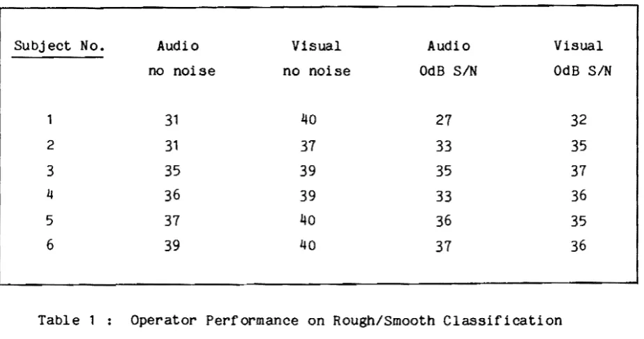
4.3.2 Rough Versus Smooth Characterizations
Had sea trials been attempted to determine the most useful approach to distinguishing man-made objects from others, the exercise would not only have been time consuming and costly, but would have required an underwater sonar sufficiently flexible to incorporate design features suggested by the trials. Instead, an air model of the underwater Classification Sonar was used. This air sonar was the first dual demodulation sonar described in section 3.3, which swept from 100 to 50 kHz in a user selectable sweep period. Initial experimentation suggested that the most useful discrimination criterion (in terms of both operator and computer characterization capablli ty) was that man-made obj ects have essentially smooth surfaces wi th relatively few reflecting pOints, while naturally