Influence of Image Pre processing to Improve the Accuracy in a Convolutional Neural Network

www.editada.org

_______________________________________________________________________________________

© Editorial Académica Dragón Azteca S. de R.L. de C.V. (EDITADA.ORG), All rights reserved.

Influence of Image Pre-processing to Improve the Accuracy in a Convolutional Neural

Network

Felipe Arias Del Campo1_{, Osslan Osiris Vergara Villegas}3_{, Vianey Guadalupe Cruz Sánchez}2_{, Lorenzo Antonio}

García Tena3_{, and Manuel Nandayapa}3

1 _{Universidad Autónoma de Ciudad Juárez, Instituto de Ingeniería y Tecnología, Doctorado en Ciencias en}

Ingeniería (DOCIA)

2 _{Universidad Autónoma de Ciudad Juárez, Instituto de Ingeniería y Tecnología, Departamento de Ingeniería}

Eléctrica y Computación

3 _{Universidad Autónoma de Ciudad Juárez, Instituto de Ingeniería y Tecnología, Departamento de Ingeniería}

Industrial y Manufactura

[email protected], {overgara, vianey.cruz, lorenzo.garcia, mnandaya}@uacj.mx

Abstract. Convolutional neural networks (CNN) have been applied in different fields including image recognition. A CNN requires a set of images that will be used to teach to classify it into specific categories. However, the question about how image pre-processing influences CNN accuracy has not yet been answered bluntly. This paper proposes the application of pre-processing methods for the images’ feed to a CNN in order to improve the accuracy of the classification. Two methods of pre-processing are evaluated, quantization and sharpness enhancement. Quantization carries out at 7 levels, and sharpness works with four levels using the discrete wavelet transform. The tests were implemented with two CNN models, LeNet-5 and ResNet-50. In the first part of this paper the methodology and description of the CNN models, as well as the data set are presented. Later the descriptions of the experiments are presented. Finally, it is shown how the proposed method achieved an improvement on the accuracy compared with the results obtained with the images with no modification. The proposed pre-processing methods had an improvement between 1.35 and 3.1% on the validation accuracy.

Keywords: Image pre-processing, CNN, quantization, sharpness enhancement, wavelet transform.

Article Info

Received Sep 26, 2018 Accepted Sep 11, 2019

1

Introduction

The ability to recognize or classify objects is something that comes natural for a human being, however, for a computer this capability is not a simple task, even with the recent advances in computer vision (CV) techniques. There are two basic elements that are required to use a computer for the task of object recognition: the object’s digital representation, and the algorithm to carry out detection and classification.

The digital representation can be a picture or a video, either in real time or pre-recorded. If the task is to recognize objects in a video, the analysis is to be applied over a specific frame or set of frames. Therefore, the recognition process can always be seen as the detection of objects in a digital image (thinking of each video frame as a simple digital image).

89

the algorithm, this is called supervised learning. The second type of training only requires the digital image, leaving the task of determining the object’s category to the algorithm, this is called unsupervised learning.

Object recognition techniques using DL methods have been gaining more interest because they outperform traditional algorithms. The increasing number of available data sets composed of images, that are used to teach computers to recognize objects, offer researchers a variety of data to use for the learning process [1].

Convolutional neural networks (CNN) are part of the DL methods, they are an extension to the multilayer neural networks (MLN). Since their introduction with the LeNet5 architecture, by Yan Lecun in 1998 [2], they have been used extensively for object recognition in both, images and videos. In order to use a CNN to solve a problem it is necessary to create a model and train it. A CNN learns how to recognize objects by presenting a set of images, that represent a sample of the universe of objects to classify, and the expected classification value for each one of them. Then, the model learns to classify the input images, but it is also able to classify images that have not been presented, this is known as a generalization, and this is one of the most relevant features of the artificial neural network models nowadays.

One of the challenges to train a CNN is to find the right set of images (known as data set). Depending on the nature of the problem, the set of images may be large, or small; for example, when working with medical images, it is common the use of small sets of images [3], [4]. A large data set provides many samples, from which the CNN can extract many distinctive characteristics, this helps to improve the network’s performance, and increase its capability to generalize. The work of [5] documented how the size of the training set impacts the classification capability using two different neural network models, SW-Net and U-Net [5].

The difference in the achieved performance of a CNN trained with a larger data base can be inferred of the results from other published works. For example, the work of [6] used two data sets, the MNIST (Modified National Institute of Standards and Technology) with 60,000 images, and the RTSD (Russian Traffic Sign Dataset) with 10,400 images to train and evaluate the same model, achieving an accuracy of 99.45% and 97.3% respectively. The differences, according to the authors, are associated with the number of images that were used to train each model. On the other hand, in [7] , the authors used a data set with only 3,753 medical images to train a CNN model to classify RGB images in order to recognize different types of cancer, achieving an accuracy of 94.2%, while the results of previously cited works were below 90%. The work proposed by [8] used 10,728 images to train the marine organism classification model, reporting a 92% of accuracy, top of 91% of the best of the reference values from other cited methods.

A method used to increase the data sets with low number if images is the data augmentation, by applying transformations like rotation, shifting, mirroring, brightness change, etc., over the images [3], [4], these techniques are used to improve the generalization of the trained model like in LIDAR systems [9].

A CNN is composed of several layers, being the first a convolutional filter that is applied over the input images. After this layer, depending on the model, it is possible also to have an activation function layer and then a MaxPooling function layer, the latter being a method to reduce the image size by picking the maximum value within a moving window. This set of layers can be found sequentially repeated, or in parallel for some models. The purpose of those layers is to create a feature map of the input image. Connected to the feature map extraction layers is a classification neural network, this classifier starts with a flattening function that transforms the feature map into a vector. The feature map is commonly presented as a bidimensional or tridimensional array. The vector is then feed-forwarded to a densely connected neural network, it will perform the classification of the feature maps, providing the actual CNN output value [10].

A method to improve the quality of the input images, or enhance the information, consisting on the application of digital filters (DF). The DF can be used to improve visibility of the image, or reduce noise, to facilitate the detection of defining features, a few examples of those filters are the changes on brightness, contrast or sharpness. Another type of DF performs a transformation of the image color space, from RGB (Red, Green and Blue) colorspace, that encodes the image intensity by the level of the red, green and blue colors (this model is used to store images that are displayed by light emitting devices), to color spaces like YUV, that encode the information by separating the chroma from the intensity, in different channels.

90

these two models were chosen because one of them represent a low performance (LeNET-5) model and the other a high performance (ResNET50) architecture; this difference is used to identify the influence of the pre-processing stage on the CNN architectures with different performance inherent to its architecture.

The rest of the paper is organized as follows, section 2, explains the characteristics of the data sets and the CNNs models used for the evaluation of the proposed preprocessing methods; section 3, explains the experiments performed over the data sets, and the results obtained with each method; finally, section 4, presents conclusions and proposes further work.

2

Methodology

In this section, the information about the hardware used to run the experiments, a description of the images data set, the CNN models evaluated, and the different preprocessing methods that were applied to the images are presented.

2.1Hardware

The development system was a desktop computer with a solid-state hard drive (that speedups the memory pagination operations and the data set loading), running Windows 10 64 bits, with an Intel i7-4790K microprocessor (not overclocked) with 20Gb of RAM, with an NVIDIA GeForce 1050 Ti GPU, with the CUDA 10.1 drivers and its requisites installed. We considered this hardware is enough to run the CNN models.

2.2Image Data Set

To evaluate the performance of the proposed kernels, it was decided to use two small data sets. The 102 Category Flower [11] data set, with images of 102 categories of flowers, and the Belgium Traffic Signals [12], with traffic signals from Belgium. The size of the data set is relevant because small data sets tend to offer poor performance for the CNN and can be used to train the model on a computer without high-end peripherals.

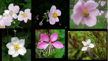
The 102 Flowers data set contains 8,189 images of 12 different flowers as it is shown in Fig. 1, the images have different sizes that vary from small (500 × 500 pixels) to big (1024 × 500 pixels). Some of these pictures have one flower and others more than ten, with a very complex background. From the 8,189 images, 75% was used for training, and the rest was used for validation, resulting on 6,141 to train and 1,937 to evaluate the model. Because of the architecture of the CNNs, the images were scaled to 32 × 32 pixels when they were processed with the LeNET-5, and to 64 × 64 for the ResNET-50.

Fig. 1. Example of the images in the 102 Flowers dataset.

The Belgium TS dataset contains 61 different traffic signals as it is shown in Fig. 2, cut from natural images, that means that they have defects as focus errors, obstructions and deformation (because of the different perspectives). The data set was split in two, with 4,638 training, and 2,583 testing images. The images in the data set are presented in color and were taken from different angles, the background is preserved to some extent, they come in different sizes, the smallest are 36 × 34 pixels, while the biggest are 230 × 334 pixels. The categories are not balanced, some have just 6 images and others up to 317 images.

91

Fig. 2. Traffic symbols from the BelgiumTS data set.

(a) (b)

Fig. 3. Two images representing a speed limit signal belonging to the same category, however each with a different meaning, a) 50 kph, and b) 70 kph value respectively.

2.3CNN Architecture

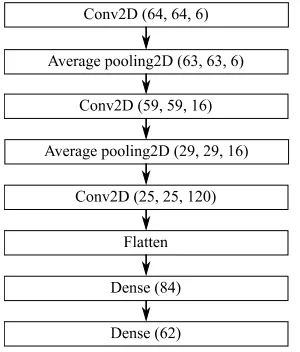
The LeNet-5 model was proposed by [2], and was implemented with TensorFlow 1.14, the open source library developed by the Google Brain team and extensively used for machine learning applications. The LeNet-5 model was chosen because it is simple, well known, and used as a starting example for learning about CNN. The simplicity of the model facilitates the visualization of the effects for the different kernels that were used in experiments. This is possible because there are fewer elements involved in the network operation. There are three convolution layers and two pooling layers in the LeNet-5 (Fig. 4), they are organized with one pooling layer after a convolution, the purpose of these five layers is to create a feature map of the input image. The convolution layers are used to extract features from their inputs, and the pooling layers perform a down sampling of the results. The feature map is a fully connected layer, acting as a classifier. The feature map passes through a flatten layer, before passing the result vector to the classifier. The classifier is a SoftMax layer that translates the output of the classifier into a vector of probabilities, that contains output for each possible class in the data set.

Fig. 4. The architecture for the LeNET-5 CNN.

92

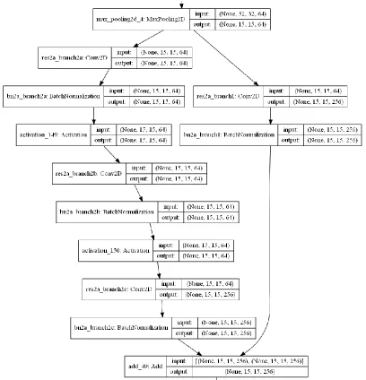
a layer with some layers below (Fig. 5), then the input and the generated feature map are used to calculate a residual, which is passed to several similar blocks in series. The complete implementation has 16 blocks. The feature map is feed to a classifier that generates the output vector, using a dense layer with a SoftMax activation function. Fig. 5 shows only the first block, each progressive block increases the number of inputs, by a power of two, the initial block has 64 inputs and ends with 256. The number of parameters in this model required more GPU memory than the currently available in the already described hardware, therefore, it was needed to reduce the size of the training batch to 8, and the input images were scaled down to 64 × 64 pixels.

Fig. 5. Fragment of the ResNet-50 showing the first branch where the feature map is obtained, and later the same input is used to calculate a residual, that is passed to a similar layer, repeating the process.

2.4Pre-processing Methods

The data sets of images were loaded in RGB format. The digital images in RBG store its information in three planes, one for each color, where the color intensity is in the range between 0 and 255 levels. Each value is normalized by dividing it by 255, producing an intensity range from 0 to 1, for each color, this value is used as the input for the CNN.

93

quantization was done by using the K-means algorithm that creates clusters from the different colors in the image, it uses the Euclidian distance of the different colors to assign them to a single cluster. The quantization preprocessing was done by using different quantization levels; 2, 4, 8, 16, 32, 64 and 128.

As well, the discrete wavelet transform (DWT) was used to separate the image in four frequency components, the low-pass filter generates the scaled component (LL), which represents the original image scaled to half its original dimensions, the high-pass filters, applied in combination with the low pass, yields the detail or local changes in brightness including three components (LH, HL and HH). Because the high frequency components of the DWT represent the local changes of brightness, they can be used to increase the sharpness of the image, multiplying them by a scaling factor, and then reconstructing the image using the inverse DWT (IDWT). This method has been used previously to enhance medical images [14], and satellite images [15], among other applications. In this work, the high frequency components (LH, HL and HH) were multiplied by a scale factor, varying in a range between 1.02 and 1.08 in steps of 0.02, those values were found to be in the range that improved the network performance, the LL component was left with its original value.

Because the RGB color images are represented in 3 color planes, it is not possible to apply the 2D DWT (bidimensional DWT), as it operates over one plane. To solve this problem, the image is first changed to the 𝑌𝑈𝑉 encoding format, where the luminance is represented by the 𝑌 plane and the chroma by 𝑈 and 𝑉 [16]. The DWT is done over the 𝑌 plane, after the scaling factors are applied, and the data is reconstructed with the IDWT, the result replaces the 𝑌 plane and then the image is converted back to the RGB color space, this new image is then feed to the CNN. The pre-processing manipulation is done over each image used to train and validate the model.

3

Experiments and Results

To evaluate the two pre-processing methods (quantization and sharpness enhancement), the CNN models, LeNet-5 and ResNet-50 were implemented with TensorFlow. Each pre-processing algorithm was evaluated, changing the customization parameter, in the case of the quantization method, this parameter is the number of quantization levels, with the values 2, 4, 8, 16, 32 and 128 (high values did not give better results, so, to save time, additional levels were not included).

The experiment implied the combination of the pre-processing methods and CNN models with the selected data sets. Because different values in the hyperparameters can also change the performance of the network can change too. They were set to the same value in an attempt to reduce the differences. Both CNN models were trained by using the SDG optimization algorithm, with a learning rate of 0.0001; to prevent overfitting, this value yields into a slow training phase, however, it was found that with larger values the ResNet-50 failed to converge. The training had an early stop callback configured to terminate the training when the delta in the loss had a difference of less than 0.01 with a patience value of 5.

During each training epoch, the best weights were saved, after the training cycle was complete (either it did not show improvement or 150 epochs were done), the best weights were loaded, and the evaluation data was used to calculate and report the accuracy metric. The size of the training batch was set to 8, because the limitations in the GPU RAM memory made it impossible to use larger batches in the ResNet-50 CNN. To avoid an advantage by using larger batches in the LeNet-5, it was decided to use the same value for both CNN models, it was seen during the experiments that by using larger batches, like 128, the accuracy improved by between a 2% to 10%.

Table 1 shows the accuracy values obtained with the validation set from the Belgium TS database after the CNN is trained and the best weights are loaded. The values obtained with the images without any pre-processing are in the first row (Original), the values obtained for the different pre-processing methods, are shown below. In the Belgium TS data set, the highest value in accuracy, with both CNN models, was obtained when the image was pre-processed, getting a 92.62% with quantization to 16 levels, versus 91.27% with the original image, for the LeNet-5. The ResNET-50 obtained the best performance for the quantization at 128 colors, with a value of 87.53% versus 84.44% with the image without pre-processing. For the case of sharpness enhancement, the best value for the LeNet-5 was obtained with a step of 1.02. For the case of ResNET-50 the best accuracy value was obtained with a step of 1.06.

94

quantization at 8 levels of color, while with the original images, the accuracy achieved was 27.78%. Finally, for the sharpness enhancement, the best value was obtained with a step of 1.06.

Table 1. Accuracy values in % obtained with the Belgium TS data set.

Pre-processing LeNET-5 ResNET-50

Original 91.2698413 84.4444444

Quantization 2 80.9126984 79.0079365

Quantization 4 90.3968254 84.1269841

Quantization 8 91.8650794 85.0396825

Quantization 16 92.6190476 85.3571429

Quantization 32 91.7460317 86.1904762

Quantization 64 91.5873016 83.9682540

Quantization 128 91.2301587 87.5396825

Wavelet HL, LH and HH × 1.02 92.3412698 83.8095238 Wavelet HL, LH and HH × 1.04 90.7539683 85.0793651 Wavelet HL, LH and HH × 1.06 90.7539683 85.5555556

Wavelet HL, LH and HH × 1.08 92.1825397 84.7619048

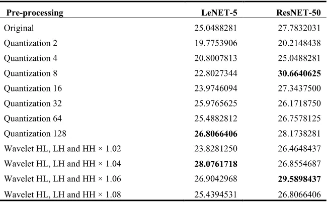
Table 2. Accuracy values in % obtained with the 102 Flowers data set.

Pre-processing LeNET-5 ResNET-50

Original 25.0488281 27.7832031

Quantization 2 19.7753906 20.2148438

Quantization 4 20.8007813 25.0488281

Quantization 8 22.8027344 30.6640625

Quantization 16 23.9746094 27.3437500

Quantization 32 25.9765625 26.1718750

Quantization 64 25.4882812 26.7578125

Quantization 128 26.8066406 28.1738281

Wavelet HL, LH and HH × 1.02 23.8281250 26.4648437 Wavelet HL, LH and HH × 1.04 28.0761718 26.8554687 Wavelet HL, LH and HH × 1.06 26.9042968 29.5898437

Wavelet HL, LH and HH × 1.08 25.4394531 26.8066406

3.1Discussion

As can be observed from Tables 1 and 2, the pre-processing of the images that are feed to a CNN affected the accuracy; the quantization provided better results than the Wavelet transform optimization, in three experiments, only with the 102 Flowers data set, and the ResNET-50 architecture, the improvement in the sharpness gave the higher accuracy value.

95

However, for the 102 Flowers data set, the best performance was obtained with an enhancement in the sharpness for the LeNET-5 model, while with the ResNET-LeNET-50 the best result was obtained using the quantization to 8 colors. The best results using the wavelet transform optimization algorithm are attributed to the fact that this data set has more complex images than the Belgium TS, the flowers have much more detail in the images, and some have complex backgrounds.

The results seem to indicate that for complex images, like the flowers, an increase in the relative difference between the element’s boundaries help to improve the CNN performance. However, if the images have more elements with homogeneous areas (color), the quantization provides better results. This makes sense considering that the quantization will increase the homogeneity of the images.

4

Conclusions

In this paper, the influence of image pre-processing to increase accuracy in a CNN was discussed. The methods of quantization and sharpness enhancement were tested with LeNET-5 and ResNET-50 models, showing that their accuracy is increased when image pre-processing was carried out. For the case of quantization 7 steps ranging from 2 to 128 color levels were tested. On the other hand, sharpness enhancement was implemented by using the DWT with four different steps.

The 102 Category Flower and the Belgium Traffic Signals small data sets were used for experimentation. The best accuracy obtained was 92.61% using LeNET-5, which is superior compared with any value obtained without pre-processing. In the end, the proposed pre-processing methods gave an improvement between 1.35 and 3.1% on the validation accuracy.

In the future, the evaluation of quantization levels between 16 and 32 will be evaluated, to try to reduce the range of the best quantization levels. Also, it will be interesting to test other CNN models.

References

1. Voulodimos, A.; Doulamis, N.; Doulamis, A.; Protopapadakis, E.: Deep Learning for Computer Vision: A Brief Review. Computational Intelligence and Neuroscience, vol. 2018 (2018), pp. 1-13. doi: https://doi.org/10.1155/2018/7068349.

2. Lecun, Y.; Bottou, L.; Bengio, Y.; Haffner, P.: Gradient-Based Learning Applied to Document Recognition. Proceedings of the IEEE, vol. 86, no. 11 (1998), pp. 2278-2324.

3. Kayalibay, B.; Jensen, G.; Smagt, P. V. D.: CNN-Based Segmentation of Medical Imaging Data. Arxiv Preprint Arxiv:1701.03056 (2017). 4. Yamashita, R.; Nishio, M.; Do, R. K. G.; Togashi, K.: Convolutional Neural Networks: An Overview and Application in Radiology.

Insights into Imaging, vol. 9, no. 4 (2018), pp. 611-629. doi: 10.1007/s13244-018-0639-9.

5. Vigueras-Guillén, J. P.; Sari, B.; Goes, S. F.; Lemij, H. G.; Van R. J.; Vermeer, K. A.; Van V. L. J.: Fully Convolutional Architecture vs Sliding-Window CNN for Corneal Endothelium Cell Segmentation. Bmc Biomedical Engineering, vol. 1, no. 1 (2019), pp. 1-16. doi: 10.1186/s42490-019-0003-2.

6. Alexeev, A.; Matveev, Y.; Kukharev, G.: Using a Fully Connected Convolutional Network to Detect Objects in Images. in 2018 Fifth International Conference on Social Networks Analysis, Management and Security (snams), 2018, pp. 141-146, doi: 10.1109/SNAMS.2018.8554685.

7. Dorj, U.; Lee, K.; Choi, J.; Lee, M.: The Skin Cancer Classification Using Deep Convolutional Neural Network. Multimedia Tools and Applications, vol. 77, no. 8 (2018), pp. 9909-9924, doi: 10.1007/s11042-018-5714-1.

8. Lu, H.; Li, Y.; Uemura, T.; Ge, Z.; Xu, X.; He, L.; Serikawa, S.; Kim, H.: Fdcnet: Filtering Deep Convolutional Network for Marine Organism Classification. Multimedia Tools and Applications (2017), pp. 1-14. doi: 10.1007/s11042-017-4585-1.

9. Caltagirone, L.; Bellone, M.; Svensson, L.; Wahde, M.: Lidar–Camera Fusion for Road Detection Using Fully Convolutional Neural Networks. Robotics and Autonomous Systems, vol. 111 (2019), pp. 125-131, doi: https://doi.org/10.1016/j.robot.2018.11.002.

10. Baldominos, A.; Saez, Y.; Isasi, P.: Evolutionary Convolutional Neural Networks: An Application to Handwriting Recognition. Neurocomputing, vol. 283 (2018), pp. 38-52. doi: https://doi.org/10.1016/j.neucom.2017.12.049

11. Nilsback, M.; Zisserman, A.: Automated Flower Classification over a Large Number of Classes. in 2008 Sixth Indian Conference on Computer Vision, Graphics & Image Processing, 2008, pp. 722—729

12. Timofte, R.; Zimmermann, K.; Van G. L.: Multi-View Traffic Sign Detection, Recognition, and 3d Localization. Machine Vision and Applications, vol. 25, no. 3 (2014), pp. 633—647

13. He, K.; Zhang, X.; Ren, S.; Sun, J.: Deep Residual Learning for Image Recognition. in 2016 IEEE Conference on Computer Vision and Pattern Recognition (cvpr), 2016, pp. 770-778, doi: 10.1109/CVPR.2016.90.

14. Rasti, P.; Daneshmand, M.; Alisinanoglu, F.; Ozcinar, C.; Anbarjafari, G.: Medical Image Illumination Enhancement and Sharpening by Using Stationary Wavelet Transform. in 2016 24th Signal Processing and Communication Application Conference (siu), 2016, pp. 153— 156

96