channel by Widom’s particle insertion method
Dezs˝o Boda1,2∗, Janhavi Giri3,4, Douglas Henderson2, Bob Eisenberg3, and Dirk Gillespie3
1
Department of Physical Chemistry, University of Pannonia, P.O. Box 158, H-8201 Veszpr´em, Hungary 2
Department of Chemistry and Biochemistry, Brigham Young University, Provo, UT 3
Department of Molecular Biophysics and Physiology, Rush University Medical Center, Chicago, IL 60612 and 4
Department of Bioengineering, University of Illinois at Chicago, Chicago, IL 60607 (Dated: December 9, 2010)
The selectivity filter of the L-type calcium channel works as a Ca2+binding site with a very large affinity for Ca2+
versus Na+ . Ca2+
replaces half of the Na+
ions in the filter even when these ions are present in 1µM and 30 mM concentrations in the bath, respectively. The energetics of this strong
selectivity is analyzed in this paper. We use Widom’s particle insertion method to compute the space dependent profiels of excess chemical potential in our Grand Canonical Monte Carlo simulations. These profiles define the free energy landscape for the various ions. Following Gillespie (Biophys. J.
94, 1169, 2008.), the difference of the excess chemical potentials for the two competing ions defines the advantage that one of the ions has over the other in the competition for space in the crowded selectivity filter. These advantages depend on ionic bath concentrations: the ion that is present in the bath in larger quantity (Na+) has the “number” advantage which is balanced by the free energy advantage of the other ion (Ca2+). The excess chemical potentials are decomposed into hard sphere exclusion and electrostatic components. The electrostatic terms correspond to interactions with the mean electric field produced by ions and induced charges as well to ionic correlations beyond the mean field description. Dielectrics are needed to produce micromolar Ca2+ versus Na+ selectivity in the L-type channel. We study the behavior of these terms with changes in bath concentrations of ions, charges and diameters of ions, as well as geometrical parameters such as radius of the pore and the dielectric constant of the protein. Ion selectivity in calcium binding proteins probably has a similar mechanism.
I. INTRODUCTION
The selectivity filter of calcium (Ca) channels, especially the highly Ca2+ selective L-type Ca channel, is thought
to have a high-affinity binding site for cations1. The filter, at appropriate pH, is rich in negatively charged carboxyl
groups similar to the binding sites of Ca2+-binding proteins. Point mutation experiments show that the filter contains
four negative charges that make the filter selective for Ca2+over monovalent cations. The energetics of this selectivity
is the main concern of this paper. We compute the components of the equilibrium free energy landscape of various ions as a function of Ca2+concentration in the bath to understand how each component contributes to selectivity.
The calculation of free energy of binding of a ligand to a receptor has drawn considerable attention in the last decades2. Though the theoretical background of free energy calculations has been known for some time3,4, their
practical use became possible with the appearance of fast computers. After the development of the first simulation methods for free energy calculations5–12, application to biomolecular systems started in the middle of the 1980s.13–18
Most free energy calculations focus on relative free energy differences between states 1 and 2. This difference is formally given by Zwanzig’s formula4
∆G=G(2)−G(1) =−kTlnhexp (−∆U/kT)i1, (1)
wherek is Boltzmann’s constant,T is the absolute temperature, ∆U is the energy difference between configurations of the two states, and the h· · · i1 denotes an ensemble average in state 1. Zwanzig introduced this procedure as
a perturbation method, where state 2 is a small perturbation to state 1. Therefore, it is called the Free Energy Perturbation (FEP) method. In practical biological applications states 1 and 2 can be far from each other, so the difference is usually computed by an integration through small steps between states 1 and 2.
In the case of Ca channels, we are interested in the binding free energy of a given ionic speciesiin the selectivity filter from a bath of given ionic concentrations:
∆Gi =Gi(filter)−Gi(B), (2)
where B denotes “bath”. The free energy Gi(B) can be obtained from Eq. 1 assuming that state 1 is the bath electrolyte and that state 2 is produced by adding an ion to the bath electrolyte:
Gi(B) =−kTlnexp −∆UB/kTB (3)
and similarly forGi(filter). This equation formally corresponds to Widom’s particle insertion method5, in which a
“ghost” particle is added to the system at uniformly distributed random locations; the energy cost of this insertion is calculated; and the Boltzmann factor is averaged in a simulation sampled over the system without the inserted particle. (That is why it is called a “ghost” particle.) Widom’s method estimates the excess chemical potential (EXCP) that describes the influence of intermolecular interactions beyond the ideal gas approximation:
µi=µTOTi −kTln Λ3i =kTlnci(r) +µEXi (r), (4)
where µi is the configurational chemical potential, Λi = h/√2πmikT is the thermal de Broglie wavelength, h is Planck’s constant, mi is the mass of the ion, ci(r) is the possibly space-dependent density (we call it concentration from now on) profile, andµEX
i (r) is the possibly space dependent EXCP. The free energyGi(B) then corresponds to the EXCP of the ionµEX
i (B). The free energy difference then reduces to the calculation of the difference of EXCPs:
∆Gi= ∆µEXi =µEXi (filter)−µEXi (B). (5)
Three very important aspects of ion binding in ion channels must be emphasized.
1. The EXCP is strongly space dependent in an ion channel and can change steeply over a wide range. The concentrationci(r) necessarily changes steeply over a wide range too. Ca2+ions, for example, can have a large
density in the filter (on the order of 10 M), while their concentration can be less than 10−6M in the bath (for
example, in biological cells). This variation must be mirrored by µEX
i (r) becauseµi is constant in equilibrium (see Eq. 4). Therefore, the binding free energy cannot be characterized simply by a number: one must calculate an EXCP profile ∆µEX
i (r) (free energy landscape) in order to properly describe the energetics of ion binding. Anything that changes the landscape will change the binding free energy. Rate constants derived from that free energy are widely used to characterize ion binding to enzymes19 and their cousins20, ion channels21. Binding
2. The other, often overlooked, property of binding free energies is that they usually depend strongly on the ionic concentrations (e.g., of Ca2+ and Na+) in the bath. In molecular dynamics (MD) simulations the binding
free energy is usually computed at infinite dilution22–24with little attention paid to the fact that experimental
measurements are usually reported over a wide range of concentrations and compositions of the bathing solutions. The ionic composition of the filter (and consequently, the EXCP) changes as the composition of that bath is changed. In the L-type Ca channel, for example, Ca2+ gradually replaces Na+ in the selectivity filter as the
concentration of Ca2+is increased in the bath from 0 to millimolar. Therefore, EXCP profiles should be reported
as functions of bath electrolyte composition so that simulations can connect to experiments.
3. Third, the structure of the binding site alone is not enough to characterize the conductance properties of the channel. (In this work, we define the binding site as the region of the selectivity filter, where the local concentration is very large.) As we have pointed out previously25–29, regions outside the binding site, where
the ionic concentrations are very small (depletion zones) are equally important in determining the permeation properties of the channel (as they are in determining properties of transistors30). We can look at the permeation
pathway as resistors in series, where a slice of the channel along the axis corresponds to a resistor. If the concentration is depleted in such a slice, the resistance in that slice is large. Consequently, the resistance of the whole channel becomes large too. The depletion zones are reflected in the EXCP profiles. The energetics of the EXCP profiles then provides useful information about the formation of depletion zones and the conductance properties of the channel. This is especially important because the current flowing through the channel at various bath concentrations is the primary experimental variable to compare with simulations or theories and also responsible for many biological functions.
The Widom method is frequently overlooked in biomolecular simulations probably because particle insertion is inefficient in dense systems with the explicit water usually used in simulations of biological systems. In this work, we use a simple implicit-water model for the Ca channel that has been successful in qualitatively reproducing experimental data such as the micromolar Ca2+ block of Na+ current and other mole fraction effects in mixtures of various ions
in the L-type Ca channel27,28,31–34. In our reduced channel model, the terminal groups of the four glutamate side
chains (EEEE) are treated as mobile structural ions and the polarization properties in the channel are tuned by adjusting the dielectric constant of the channel protein31. Competition of ions for space in the highly-charged and
crowded selectivity filter is the main driving force behind this selectivity, called the charge-space competition (CSC) mechanism35,36.
In this study, this reduced channel model is studied using equilibrium Grand Canonical Monte Carlo (GCMC) simulations31,37–39and the EXCP profiles are computed with Widom’s particle insertion method5,9(see the Appendix).
Following the recipe of Gillespie40, we decompose the EXCP into various terms (volume exclusion, electrostatic term due to ions, electrostatic term due to dielectrics, and a self term due to the dielectric barrier) and study how these components contribute to selectivity. Using a model of the ryanodine receptor (RyR) calcium channel that both reproduces and predicts experimental data, Gillespie40showed that RyR selects Ca2+over monovalent cations because
Ca2+ ions are screened (coordinated) better by the four aspartates of the selectivity filter. The RyR model does not
include dielectric interfaces, which we have shown gives the L-type calcium channel substantially larger Ca2+affinity
than RyR31. This paper builds on the work of Gillespie, not only by including dielectric interfaces, but also by
analyzing the effect of changing the pore geometry on the energetic components of selectivity.
II. MODEL
In our model, most of the atomic structure of the calcium channel is reduced to a coarse-grained geometry (Fig. 1A). The channel protein is represented as a continuum solid with dielectric coefficient ǫpr. The three dimensional
body of the protein is obtained by rotating the thick line in Fig. 1A about ther = 0 axis. The protein thus forms an aqueous pore that connects the two baths. Water in the baths and pore is described as an implicit solvent that is a continuum dielectrics with uniform dielectric coefficient ǫw= 80. The central cylindrical part of the pore (with
radiusR= 3.5−4.5 ˚A and length 10 ˚A) forms the selectivity filter that includes the only atoms of the protein that are treated explicitly. These atoms are eight half-charged ‘oxygen ions’ O1/2− (Fig. 1B,red spheres) representing the charged terminal groups of the four glutamate residues of the EEEE locus. The structural oxygen ions are confined to the selectivity filter (their centers are in the regionr ≤R−1.4 ˚A, |z| ≤3.6 ˚A), but they can move freely inside the filter. The oxygen ions ‘coordinate’ counter-ions as particles of a confined liquid; their arrangement in Fig. 1B represents one snapshot of the millions of configurations sampled during a simulation.
Ions are restricted to the aqueous space of the model and cannot overlap with hard walls in the system. Fig. 1 shows only the small central region of the simulation cell. The entire simulation cell is a cylinder with typical dimensions of radius 40 ˚A and length 180 ˚A. The channel is embedded in a membrane region that excludes ions by hard walls as described before31.
III. COMPUTATION OF THE CHEMICAL POTENTIAL TERMS
In the particle insertion method developed by Widom5,9 we work with the following operation:
W(U(r)) =−kTlnDe−U(r)/kTE, (6)
where an ion is inserted in a small ∆V volume around positionr. Its interaction energy with the system is denoted by
U(r) and the brackets denote grand canonical (GC) ensemble average. Widom developed the formula in the canonical ensemble9. Following his treatment, we show in the Appendix that the same formula applies when we simulate the
whole system in the GC ensemble. The quantity W(U) depends on position through U(r), namely, on the position where we insert the test particle.
A. Energy terms
Separating the chemical potential into different terms is based on a separation of the energy of the system into different terms. The ion-ion (denoted by II) interaction energy between a ghost ion of speciesiinserted at positionr
and all the existing ions in the system is
UiII(r) =
X
α
zizαψII(r,rα), (7)
where zi is the valence of the inserted ghost ion, the indexαruns over all the existing ions in the system,zα is the valence of theαth ion, and
ψII(r,s) =1 2
e2
4πǫ0|r−s|
1
ǫ(r)+ 1
ǫ(s)
(8)
is the interaction energy between two ions with unit valences at positionsr ands, ǫ(r) is the dielectric constant at positionr,eis the electronic charge, andǫ0 is the permittivity of vacuum.
The ion-dielectric (denoted by ID) interaction energy between the inserted ion and the polarization charge induced on the dielectric boundaryBby all the other existing ions is
UiID(r) = 1 2ezi
X
α
zαψID(r,rα), (9)
where
ψID(r,s) = e 4πǫ0
Z
B
h(s,r′)
|r−r′
|dr
′
(10)
is the potential from the polarization charge at position r. h(s,r′) is the polarization charge atr′ induced by a unit charge (zα= 1) placed at positions(and vice versa).
The interaction energy between the inserted ion and the polarization charge induced onBby the ion itself is
UiSELF(r) = 1 2z
2
ieψSELF(r), (11)
where
ψSELF(r) =ψID(r,r) (12)
is the potential from the polarization charge at positionr.
The ions are modeled as charged hard spheres (HS). The HS energyUHS
The total energy change of the system produced by inserting an ion of speciesiis
Ui(r) =UiHS(r) +UiII(r) +UiID(r) +UiSELF(r). (13)
The EXCP of an ionic speciesiinserted at positionrcan be determined from
µEXi (r) =W UiHS(r) +UiII(r) +UiID(r) +UiSELF(r)
. (14)
Note that the interior of the protein and the membrane excludes ions; therefore, another potential term should be included in Eq. 13: an external potentialUWALL
i (r), which is infinite whenever an ion of speciesioverlaps with these regions or any hard wall in the system and zero otherwise. Therefore, rigorously, Eq. 4 should be supplemented with a corresponding chemical potential term µWALLi (r). Because we will show profiles averaged over the ion-accessible area, whereµWALL
i (r) = 0 (see subsection IV B), this issue is not relevant from the point of view of our discussion.
B. The components of the excess chemical potential
Now, we separate the EXCP into different terms. Such a separation is straightforward for the energy, but we have to apply such a separation with extra care in the case of the chemical potential. Any separation of the EXCP corresponding to a separation of the energy is necessarily not unique. In this paper, we propose a possible separation that is physically well based and helps to understand the energetics of selectivity, but it is not unique.
The chemical potential of an ionic species in an ideal solution is commonly defined as
µidi .sol.=kTlnci+zieφ, (15)
where φis the mean electrical potential in the solution. In this approximation, the EX term is just the interaction with the mean potential and the ions are treated as point charges.
Using this analogy, we can define a mean field (MF) term of the EXCP. In fact, we can define various MF terms depending on what the source of the potential is. The mean potential from the ions in the system is computed as
φII(r) =
* X
α
zαψII(r,rα)
+
. (16)
The potential from the polarization charge induced by these ions is
φID(r) = 1 2
* X
α
zαψID(r,rα)
+
. (17)
The third term is the potential from the polarization charge of an inserted ion at the position where the ion was inserted:
φSELF(r) = 1 2
ψSELF(r)= 1 2ψ
SELF(r). (18)
The mean potentials are computed in the simulation by inserting test charges in various positions, the corresponding potential terms are computed at these positions, and the results are averaged over numerous insertions. This is expressed by the brackets in the above equations. The corresponding MF terms of the chemical potential then are defined as
µMFIi (r) =zieφ
II
(r), (19)
µMFDi (r) =zieφ
ID
(r), (20)
and
µSELFi (r) =zi2eφ
SELF
(r). (21)
This means that we include only theUHS
i term in Eq. 6. The HS component of the chemical potential thus is defined as
µHSi (r) =W UiHS(r)
. (22)
If we subtract the HS term and the MF terms from the total EXCP, what remains corresponds to the electrostatic correlations between ions “beyond mean field” (denoted by SC for ‘screening’):
µSCi (r) =µEXi (r)−
µHSi (r) +µMFIi (r) +µMFDi (r) +µSELFi (r)
. (23)
We can see a pattern if we write this equation this way:
µSCi (r) = W UiHS(r) +UiII(r) +UiID(r) +UiSELF(r)
− µHSi (r) +µMFIi (r) +µMFDi (r) +µSELFi (r)
.
We have similar contributions in the first and the second term on the right hand side. In the first term (the Widom evaluation of the EXCP) we compute the energies corresponding to the HS, II, ID, and SELF terms and sample all the cross-correlations between these terms. The second term also contains these contributions, but in a mean field way. We subtract these from the total, so the SC term expresses all the electrostatic correlations that are not included in the MF treatment. Because many studies still use MF theories such as Poisson-Boltzmann theory or its generalization to nonequilibrium (Poisson-Nernst-Planck), it is particularly useful to explicitly evaluate this term in order to show its importance. The SC term measures the error in mean field theories.
The next step is the separation of the correlation effects corresponding to ions and induced charges in the SC term. Formally,
µSC
i (r) =µSCIi (r) +µSCDi (r), (24)
where the superscripts SCI and SCD indicate ionic and dielectric correlations, respectively. If, in the Widom method, we insert ions in the system, but exclude the dielectrics, we can estimate a term that contains only the ionic correlations and excludes all terms involving dielectrics: W UHS
i (r) +UiII(r)
. If we follow the pattern in Eq. 24 and subtract the corresponding MF term, we obtain the SCI term as a leftover:
µSCIi (r) =W UiHS(r) +UiII(r)
−µHSi (r) +µMFIi (r)
. (25)
The SCD is then whatb is leftover; it is obtained simply from Eq. 24. All these terms can be illustrated as
EX
z }| {
HS + MFI + SCI
| {z }
ION
+ MFD + SELF + SCD
| {z }
DIEL
. (26)
C. Energetics of ion selectivity
Because the system is in equilibrium, the chemical potential is the same in the bath and in the channel:
µi =kTlnci(B) +µEXi (B) =kTlnci(r) +µEXi (r). (27)
The EXCP in the bulk (µEX
i (B)) that corresponds to prescribed ionic concentrationsci(B) is calculated using the Adaptive Grand Canonical Monte Carlo (A-GCMC) method of Malasics and Boda41,42. If we define the difference
(see Eq. 5)
∆µEXi (r) =µEXi (r)−µEXi (B), (28)
we obtain
∆µEXi (r) =kTln
ci(r)
ci(B)
. (29)
an additional sampling procedure ‘on top’ of the normal GCMC simulation. The right hand side (the concentration) is computed in the GCMC simulation in the usual way as an ensemble average. Although the EXCP could be calculated from the GCMC simulation without the Widom sampling, the particle insertions are necessary to compute the components of the EXCP.
We can define the differences between the channel and the bulk (B) not only for the excess term, but also for every term introduced above:
∆µHSi (r) =µiHS(r)−µHSi (B) (30)
∆µMFIi (r) =µiMFI(r)−µMFIi (B) (31)
∆µMFDi (r) =µiMFD(r)−µMFDi (B) (32)
∆µSELFi (r) =µiSELF(r)−µSELFi (B) (33)
∆µSCIi (r) =µiSCI(r)−µSCIi (B) (34)
∆µSCDi (r) =µiSCD(r)−µSCDi (B) (35)
∆µSCi (r) =µSCi (r)−µSCi (B). (36)
The µMFI
i (B), µMFDi (B), and µSELFi (B) terms are zero because the corresponding mean potentials ( φ
II
(r), φID(r), andφSELF(r)) are defined to be zero in the bulk. The sum of the differences for the HS, MFI, MFD, SELF, SCI, and SCD terms is the difference of the excess term. Let us now summarize all these differences for Na+ and Ca2+ and
express the differences of differences:
∆∆µHS(r) = ∆µHSNa+(r)−∆µHSCa2+(r) (37) ∆∆µMFI(r) = ∆µMFINa+(r)−∆µMFICa2+(r) (38) ∆∆µMFD(r) = ∆µMFDNa+(r)−∆µMFDCa2+(r) (39) ∆∆µSELF(r) = ∆µSELFNa+ (r)−∆µSELFCa2+(r) (40)
∆∆µSCI(r) = ∆µSCI
Na+(r)−∆µSCICa2+(r) (41) ∆∆µSCD(r) = ∆µSCDNa+(r)−∆µSCDCa2+(r) (42)
∆∆µSC(r) = ∆µSC
Na+(r)−∆µSCCa2+(r) (43)
Following Gillespie40, these terms are called ‘advantages’ because a positive value of any of them favors Ca2+binding
(accumulating) by increasing Ca2+ concentration. Using Eq. 29 and these terms, we obtain:
ln
cCa2+(r)
cNa+(r)
= ln
cCa2+(B)
cNa+(B)
+∆∆µ
EX(r)
kT , (44)
where
∆∆µEX(r) = ∆∆µHS(r) + ∆∆µMFI(r) + ∆∆µMFD(r) + ∆∆µSELF(r) + ∆∆µSCI(r) + ∆∆µSCD(r). (45)
In Eq. 44, the left hand side is called ‘binding selectivity’ because it expresses the degree to which Ca2+ is favored
over Na+at locationr. The corresponding term on the right hand side with the bulk concentrations is called ’number
advantage’ because it expresses the advantage that one ionic species has from outnumbering the other ionic species in the bulk. If ∆∆µEX
i (r) were zero, the channel would not be selective at all. The ratio of ion concentrations would be the same in the channel as in the bulk. The energetic advantage terms on the right hand side of Eq. 45 describe to what degree each term contributes to the binding affinity of Ca2+ over Na+, i.e., how each term contributes to this selectivity.
IV. METHODS
A. Grand Canonical Monte Carlo simulations
MC simulations using Metropolis sampling are performed in the GC ensemble31,37–39. This ensemble, as described
Ca2+ vs. 30 mM Na+). MC moves include (1) small displacement from the old position (for sampling regions with
large densities; this is the only kind of attempt used for the oxygen ions in the selectivity filter); (2) changes to a new position selected randomly from a uniform distribution anywhere in the cell (used for sampling regions with gas-like densities such as in the baths); (3) moving a particle from a position in the selectivity filter to a position in the baths, or vice versa; this move prefers particle exchanges between certain subvolumes and thus the acceptance test includes the subvolume ratio to prevent statistical bias43; (4) insertion/deletion of individual ions (chemical potentials
of individual ions are determined by the A-GCMC method of Malasics and Boda42) (5) insertion/deletion of a neutral
group of ions (e.g., Na++Cl− or Ca2++2Cl−); (6) particle insertions or deletions analogous to (5) but involving subvolumes of the simulation cell that we want to sample more intensely (in particular, the selectivity filter)33. Only
cation insertions or deletions are applied in these subvolumes, Cl− ions are still inserted/deleted into/from the whole simulation cell. These attempts are applied randomly with predefined probabilities. Changing these probabilities does not change the final result; it only influences the speed with which the simulation converges to the final result. The typical length of a GCMC simulation is 5×10⁸sampled configurations (attempts).
The acceptance tests for new particle configurations involve the total electrostatic energy of the system, as described in section III A. Computation of the energy terms involving dielectrics (UiID(r) andUiSELF(r)) assumes the compu-tation of the polarization surface charge h(r,s) induced on the dielectric boundaries. We compute the polarization charge using a boundary element method that we have called ‘induced charge computation’ (ICC)31,44. The Poisson
equation with boundary conditions is transformed into an integral equation and solved by surface discretization. For a given dielectric geometry, the coefficient matrix produced by the discretized integral equation does not depend on the ion configuration. It is inverted at the beginning of the simulation and used repeatedly (millions of times) during the simulation to determineh(r,s). Vectors of discretized induced charge for varied ion configurations are computed thereafter by a matrix-vector multiplication.
B. Numerical implementation of the Widom sampling
To compute the space-dependent EXCP profiles with Widom’s particle insertion method5,9(see the Appendix) we
have constructed a two-dimensional grid shown in Fig. 1A. Because the system is rotationally symmetric, we defined the subvolumes described in the Appendix as a function of only two variableszandr. In the channel we used squares of width 0.5 ˚A, while outside the channel near the channel entrances we used squares of width 2 ˚A. These squares correspond to rings in three dimensions. In the two baths we used large cylinders far from the hard walls of the system. We inserted test particles into these rings with equal probabilities. Thus, we insert particles into the rings in proportion to their cross sectional area in the (r, z)-plane instead of their volume.
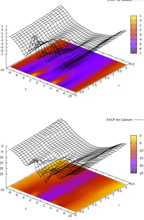
Figure 2 shows ∆µEX
Na+(z, r) (part A) and ∆µEXCa2+(z, r) (part B) for the state point that we use as an example throughout our paper: R= 3.5 ˚A,ǫpr = 10,cNa+(B) = 30 mM,cCa2+(B) = 1µM. This is the case that corresponds to the IC50 of the experiment of Almers and McCleskey45,46: 1µM Ca2+ reduces the current of 30 mM Na+ to half
of that measured in the absence of Ca2+. As we have pointed out27, our model with the geometrical parameters used in this paper and protein dielectric coefficientǫpr = 10 is able to reproduce this experimental result. At these bath
concentrations, the filter binds about the same amount of Na+and Ca2+, the amount of Na+being half of that bound
if Ca2+ is not present in the baths. Therefore, Na+ current is half the current in the absence of Ca2+. Ca2+ions do
not carry significant current in the case shown in Fig. 2, because depletion zones are formed at the filter entrances in the density profile of Ca2+. We have previously used the integrated Nernst-Planck equation to quantify how these
depletion zones form high-resistance elements along the ionic pathway in a simplified situation27. Peaks in Figure 2 correspond to these depletion zones (where ci(r) is small,µEX
i (r) is large). The ridges at|z| ≈5 ˚A represent these depletion zones, while the valley in the center of the filter represents the binding site for the ions.
Because it is quite difficult to distill relevant information from such landscapes and because we are primarily interested in the behavior of the system along the ionic pathway, we average these profiles over ther-dimension:
∆µEX i (z) =
2
R2 min
Z Rmin
0
r∆µEX
i (z, r)dr. (46)
Similar expressions apply for all the other chemical potential terms. When averaging, one must be careful. We need to average the profiles for Na+ and Ca2+ over the same range ofr in order to compute the difference ∆∆µEX(z) =
∆µEX
Na+(z)−∆µEXCa2+(z) properly. The range over which we average is the range that is accessible to the center of the largest ion: Rmin =R−Rlargest ion. In this way we can compare EXCPs for the two ions over a cross section that
both ions occupy. We will drop the overline from now on to simplify the notation.
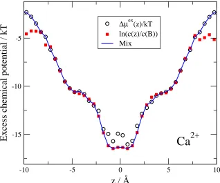
Equation 29 makes it possible to check the self-consistency of our simulations. Figure 3 shows both the profile ∆µEX
(outside the central binding site) the Widom-sampling works better. In these regions, sampling of Ca2+concentration
can be poor. In some volume elements, Ca2+ concentration can be zero; therefore, the logarithm diverges making
the average over the cross section in Eq. 46 diverge too. The Widom-sampling, on the other hand, can be poor in regions of large concentrations because particle insertion is problematic in high-density regions. Therefore, we mix a ∆µEX
Ca2+(z)/kT profile from these two functions. We define a central region where we use ln (ci(r)) (|z| = 3 ˚A in Fig. 3). We define another region outside the central region where we use Widom sampling to obtain ∆µEX
i (r). The profiles shown from now are mixed in this way. The two kinds of profiles are practically identical for Na+ions (data
not shown), because sampling is much better for Na+ than for Ca2+.
V. RESULTS
We will present our results using the point (R = 3.5 ˚A, ǫpr = 10, cNa+(B) = 30 mM, cCa2+(B) = 1 µM) as a reference point. Then, we will show the effects of changing cCa2+(B), ǫpr, filter radius (R), and the radius of the monovalent cation on the chemical potential profiles.
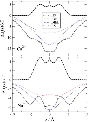
Figure 4 shows the chemical potential terms (compared to bulk) introduced in Eqs. 29-36. The EX term is much deeper for Ca2+ than for Na+, but this difference is necessary to overcome the large number advantage of Na+ over
Ca2+. The EX term is the sum of all the other terms shown in Fig. 4. This division shows how this large (free)
energetic advantage for Ca2+ decomposes into different contributions, which we describe in detail below.
The HS term describes the free energy that is necessary to insert a neutral hard sphere (with the same diameter as the corresponding ion) into the system. This term is repulsive and has similar magnitude for Ca2+and Na+ because
these two ions have similar size. The HS profiles have large peaks more or less where the oxygen concentration profiles have peaks (|z| = 3.6 ˚A), namely, where the probability that an inserted particle overlaps a particle already in the system is the largest.
The SELF term is the consequence of a dielectric penalty of an ion passing through the channel; it measures the interaction of the ion with the polarization charge induced by the ion itself.47,48 This term is positive for both ions
because the ions induce repulsive charge on the dielectric interface. This dielectric penalty is four times larger for Ca2+ than for Na+.
The MF terms describe the interaction of an inserted ion with the mean electrostatic potential. The mean electro-static potential is averaged over the millions of sampled configurations and is related to the average ionic concentration profiles (and, thus, to the EXCP profiles) through Poisson’s equation. Thus, the MF terms describe the channel’s ability to attract cations electrostatically in an average manner. The mean potential is negative because the channel is not charge neutral (it is net negative): cations are unable to neutralize the oxygen ions perfectly because the channel is narrow and crowded. The balancing charge is outside the channel.
The MF terms can be split into the MFI and MFD terms depending on the source of the potential (MFI from ions and MFD from dielectric induced charge). The MFI profiles follow the variation in the profile of the ionic charges,
P
izieci(r). Peaks in oxygen ion profiles produce minima in the MFI profiles. The MFD profile follows the variation of the induced charge on the dielectric interface: the induced charge is negative in the filter (because the net charge of the filter is negative) and it changes smoothly going outward from the center of the channel (see Fig. 11 of Boda et al.31). The induced charge is positive on the outer surface of the protein. Although the net amount of induced charge is zero on the whole surface of the protein due to Gauss’s law, the mean potential it produces (MFD) inside the channel is negative. The MFI and MFD terms have similar magnitude at this value of the protein dielectric constant. The MFI and MFD terms together (MF term) overcome the repulsive SELF term, but the electrostatic terms beyond the MF terms (SC) are crucial to produce the deep excess terms resulting in the strong Ca2+versus Na+ selectivity.
The SC terms describe electrostatic correlations beyond the MF terms. Formally they can be interpreted by the difference
−kTlnDe−ψ/kTE− hψi, (47)
where ψ denotes some kind of energy in the system. (Note that this equation is a simplification for pedagogical purposes. The exact computation of the SC terms is given in section III B.) In particular, the SCI term is related to the ability of the local surrounding electrolyte to screen the charge of the ion inserted into a given position in the system. (This screening should not be confused with screening by water, which is represented by the dielectric coefficient.)
ideality. This term is commonly (and approximately) described by the textbook theory of Debye and H¨uckel (this theory ignores the HS term and thus is in error under many important conditions).
To understand the SCD term, first we consider the MFD term which represents the potential from the average induced charge (second term in Eq. 47). The induced charge, however, varies as ions change positions in the channel during MC sampling. A successfully inserted (no overlap) test ion will then experience the potential of the induced charge of a given ionic configuration. Different successfully inserted ions will experience different forces. The average over all these configurations is computed by the Widom sampling (first term in Eq. 47). The difference of these two terms defines the SCD term.
The SCI term in Fig. 4 has a non-monotonic behavior. It has a positive maximum where the MFI profile has a minimum. At these positions it is more difficult for the surrounding ions to screen the inserted ion compared to the average. The SCD term can be very different from the mean (MFD) as seen in Fig. 4: the SCD term is deeper (more attractive) than the MFD term under the given conditions. Note that the effect of the charge induced by the inserted test ion itself is not included in the SCD term; that is the SELF term.
Different insight can be gained if we separate the EXCP into components corresponding to interactions with ions (ION=MFI+SCI) and to interactions with induced charge (DIEL=SELF+MFD+SCD), see Eq. 26. The results are shown in Fig. 5. Interestingly, the ION term is a non-oscillating function ofz(apart from the one minimum), while its components (MFI and SCI) are oscillating. The DIEL term is also non-oscillating. Fig. 5 shows that at this value of
ǫpr the DIEL term is even deeper than the ION term. The ions occupy positions in the filter with higher probability
with which they minimize free energy. The number of such configurations is limited. Therefore, the SCI term has its limitations in drawing more ions into the filter. It is the DIEL term that has a large additional attractive effect ifǫpr
is small.
Fig. 5 gives the impression that it is the HS term and volume exclusion effects between ions that produce the oscillatory behavior of the EXCP and thus the peaks in the ionic profiles. This impression is false, however, because large density has its consequences not only directly in the HS term, but also indirectly in the electrostatic terms. The cations try to find positions between the oxygens with the best possible screening. Together with the effects of confinement from the pore wall and the oxygen ions, this results in layering in the density profiles. The oscillations in the SCI and MFI profiles reflect this phenomenon.
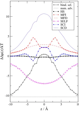
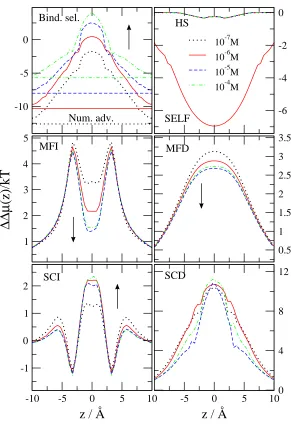
In the next step we take the differences of the ∆µi(z) functions shown in Fig. 4 (Eqs. 37-43) and express binding selectivity and the advantages stemming from the different terms (Eq. 45). Figure 6 shows these ∆∆µ(z) functions. The number advantage favors Na+over Ca2+because there is much more Na+in the bulk than Ca2+(ln(10−6/0.03) =
−10.3, a constant). This expresses the higher probability of Na+ ions diffusing in the vicinity of the channel relative
to Ca2+. The binding selectivity curve equals the number advantage curve in the baths outside the channel. Inside
the channel, however, the binding selectivity curve increases and in the binding site (center) of the selectivity filter it is positive, meaning that this site favors Ca2+ over Na+ under the given conditions. To overcome the large number
disadvantage, a large EXCP advantage (∆∆µEX(z)) is needed for Ca2+.
Figure 6 shows how this advantage splits into different terms. The HS advantage is close to zero because the size of the two ions is very similar. Both the MFI and MFD terms favor Ca2+, as expected, because the double charge of Ca2+ has double the interaction energy with the MF potentials (φII(z) and φID(z)) compared to Na+. The most
favorable term for Ca2+ is the SCD term. The SCD term is so large that it (together with the MFI, MFD, and SCI
terms) can overcome the unfavorable SELF term. The self term is the only term that is very unfavorable for Ca2+
because Ca2+has four times the interaction energy with its own repulsive induced charge than Na+ does.
Next, we analyze the effect of various parameters on ion selectivity and the role of the different advantage terms in the change of selectivity. First, we consider the Ca2+ titration experiment performed by Almers and McCleskey45,46
and changecCa2+(B) in the fixed 30mM Na+ background. Figure 7 shows the various advantage terms for different values of the bulk Ca2+ concentration. (Note that different advantage terms will be shown for different problems
in Figs. 7-11 depending on which term is more important for a given case.) The basic conclusions are similar to those drawn by Gillespie40 for the RyR Ca channel in a similar experiment. Binding selectivity increases (becomes
more favorable for Ca2+) asc
Ca2+(B) increases (the Na+ number advantage decreases). The MFI and MFD terms decrease with increasing cCa2+(B) because the channel becomes more charge neutral; Ca2+ ions are more efficient in neutralizing the oxygen ions. Therefore, the decrease of the MF terms is the main reason of the saturation of selectivity at large Ca2+ concentrations. The SCI and SCD terms change less with increasingc
Ca2+(B), while the HS and the SELF term do not change at all.
The Ca2+ versus Na+ selectivity of the model channel can be characterized by the Ca2+ concentration at which the number of Na+ ions in the filter is half of that in the absence of Ca2+. As we have shown before27,28,34, this value
coincides with the IC50 value with which selectivity is characterized in experiments.
In a series of publications27,28,31,32,34we have shown that the shape of the titration curves (average number of Ca2+
and Na+ ions in the filter as functions of log
10[cCa2+(B)]) is similar in different conditions: Ca2+ gradually replaces Na+ in the filter as c
namely, at whichcCa2+(B) this replacement occurs. The titration curves are shifted whenever we change the radius of the filter (Fig. 2 of Ref. 32); the length of the filter (Fig. 6 of Ref. 34); the dielectric coefficient of the protein (Fig. 8 of Ref. 31); the concentration of the background Na+ (Fig. 6 of Ref. 28); the radius of the monovalent cation (Fig.
7A of Ref. 28); or the radius of the divalent cation (Fig. 7B of Ref. 28). Changing any of these parameters changes the energetics of the competition between the two cations, and, consequently selectivity.
The CSC mechanism states that the selectivity filter favors Ca2+because it is more efficient at balancing the charge
of the oxygen ions than Na+. It provides twice the charge in the same excluded volume. In this picture, the fact
that the filter is crowded has a special significance. All the parameters listed in the preceding paragraph influence the ionic density in the filter somehow, and, thus, they influence the strength of the competition between cations for the limited amount of space available in the filter. The radius and length of the filter, for example, change the volume of the filter, and, thus, ionic density. The smaller dielectric coefficient of the protein acts to attracts more cations into the filter thus making it more crowded.
Excluded volume obviously is a dominant feature of selectivity filters. Thus, it may seem counter-intuitive that Ca2+ versus Na+ selectivity does not depend on the HS term very much. This is because the HS terms express the
direct effect of the steric exclusion of the ions on their abilities to find space in the filter. If two ions have the same size, these direct effects are the same. The crowded nature of the selectivity filter, however, has a profound indirect effect on the electrostatic parts of the EXCP. Because the filter is crowded, ions have difficulty finding space in it. The filter, therefore, is never charge neutral; due to confinement and limited space, cations within the filter can only partially balance the negative oxygen ions. Some of the balancing charge is outside the filter. The resulting negative filter produces a free energy well for the cations. In this large-density negatively-charged environment, many-body ionic correlations are very important, as shown by the SC terms.
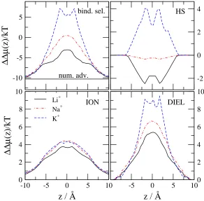
Figure 8 shows the dependence of our results on the protein dielectric coefficient, ǫpr, relative to the reference
condition ofR= 3.5 ˚A,cNa+(B) = 30 mM,cCa2+(B) = 1µM. Because the bulk concentrations are fixed, the number advantage is the same for all values of ǫpr. Binding selectivity, however, increases (the channel becomes more Ca2+
selective) asǫpr decreases from 80. The ION term decreases with decreasingǫpr. The principal source of this decrease
is the MFI term. Whenǫpr is small, more cations are attracted into the channel as discussed in our previous work31.
The energetic explanation is that it takes energy to polarize the dielectric boundaries so the system is trying to minimize the induced charge. This is possible only by making the channel more charge neutral by attracting more cations into it. Because the channel is closer to charge neutrality at small ǫpr, the MFI advantage decreases with
decreasingǫpr.
The term that increasingly favors Ca2+ with decreasing ǫ
pr is, of course, the DIEL term. Although the SELF
term favors Na+ with decreasingǫ
pr, the other two dielectric terms (MFD and SCD) increasingly favor Ca2+ with
decreasingǫpr. This result is expected because the induced charges are larger when the difference between the dielectric
coefficients on the two sides of the dielectric interface is larger.
If we keepǫpr= 10 constant and change the radius of the filter,R, instead, we obtain the results shown in Fig. 9.
Binding selectivity increases as R decreases. The ION term changes only a little with changing R; the DIEL term, on the other hand, changes a lot. Apparently, the value ofǫpr is the first order determinant of the number of cations
attracted into the filter. The value of ǫpr determines the degree of charge neutrality of the filter, which, in turn,
determines the MFI term. The ions seem to coordinate to get efficient screening even whenRis small. The important term that determines selectivity with changingRis the DIEL term. In a more narrow pore ions are closer to the pore wall on average. Therefore, the induced charge is larger and the potential produced by it in the filter is also larger. The low dielectrics surrounding the pore focuses field lines, making the total field density in the filter larger. The filter with a smaller radius focuses the field lines even more strongly. These findings are in agreement with Fig. 3 of Boda et al.32 which shows that Ca2+ vs. Na+ selectivity is more sensitive toR whenǫ
pr= 10 than in the case when
ǫpr= 80.
If we change the size of the monovalent ion (by switching ion type to Li+, Na+, and K+, using the corresponding
Pauling radii), we obtain the results shown in Fig. 10. ca2+binding selectivity increases as the radius of the monovalent
ion increases. One of the important terms is the HS term that increases considerably as the radius of the monovalent ion increases. Ca2+ can compete more efficiently for space with the larger monovalent cations. The other important
term is the DIEL term, which has the same behavior. The induced charges are smaller for the larger ions because ion centers (where charges are) are farther from the dielectric boundary. Larger positive ions, therefore, induce less positive induced charge, leaving the total induced charge more negative. More negative induced charge favors the binding of Ca2+ as we described above.
Figure 11 shows the results for the competition of two cations of the same charge, but different size. The bath concentration of both Ca2+ and Ba2+ is the same (50 mM), so the numerical advantage of Ca2+ over Ba2+ is zero. The HS term is the main source of the large binding selectivity of the smaller Ca2+ over the larger Ba2+, while the
VI. SUMMARY
We have analyzed the energetics of selectivity for a reduced model of the L-type calcium channel in terms of various components of the EXCP. These components included those due to volume exclusion (HS) and various electrostatic terms. The electrostatic terms included the MF terms due to interactions with the average field of ions and induced charges. The terms beyond the MF terms are due to many-body correlations between ions (SCI), as well as between ions and induced charges (SCD). These correlations are crucial in the case of calcium channels, where the ionic density in the selectivity filter is very large and everything interacts with everything else strongly.
Polarization, in particular, plays an important role in the behavior of the selectivity filter of the L-type calcium channel. It makes the electric field in the filter stronger and, thus, it makes the competition between the cations stronger. In this competition, multivalent and smaller ions have the advantage in the highly-charged and crowded selectivity filter. This is consistent with experimental data on both L-type and RyR calcium channels.
Even in our very reduced model of the channel we encountered a complex picture. Different terms played different roles depending on which variable was changed: bath ion concentrations, ion charges, ion radii, pore radius, or protein dielectric coefficient. It is important to emphasize that this complexity is an automatic consequence of our model and an output of our calculations. All the terms we computed must have analogs in more detailed models of the protein and electrolyte. Therefore, it is likely that this rich behavior will be present not only in real calcium channels, but also in other carboxylate-rich binding sites like those of calcium binding proteins (e.g., calmodulin) and chelators (e.g., EDTA, EGTA).
ACKNOWLEDGMENTS
This work was supported by the Hungarian National Research Fund (OTKA K75132) and in part by NIH grant GM076013. We are grateful for a generous allotment of computing time at the MARYLOU supercomputing facility of Brigham Young University.
1
W. A. Sather and E. W. McCleskey, Annu. Rev. Physiol.65, 133 (2003). 2
B. O. Brandsdal, F. ¨Osterberg, M. Alml¨of, I. Feierberg, V. B. Luzhkov, and J. ˚Aqvist, Adv. Protein Chem.66, 123 (2003). 3
J. G. Kirkwood, J. Chem. Phys.3, 300 (1935). 4
R. W. Zwanzig, J. Chem. Phys.22, 1420 (1954). 5
B. Widom, J. Chem. Phys.39, 2808 (1963). 6
G. M. Torrie and J. P. Valleau, Chem. Phys. Lett.28, 578 (1974). 7 C. H. Bennett, J. Comput. Phys.
22, 245 (1976). 8 G. M. Torrie and J. P. Valleau, J. Comput. Phys.
23, 187 (1977). 9
B. Widom, J. Stat. Phys.19, 563 (1978). 10
M. Mezei, S. Swaminathan, and D. L. Beveridge, J. Am. Chem. Soc.100, 3255 (1978). 11 A. Warshel, J. Phys. Chem.
86, 2218 (1982). 12
J. P. M. Postma, H. J. C. Berendsen, and J. R. Haak, Faraday Symp. Chem. Soc.17, 55 (1982). 13
A. Warshel, Pontif. Acad. Sci. Scr.55, 60 (1984).
14 B. L. Tembe and J. A. McCammon, Computers & Chemistry
8, 281 (1984). 15
C. F. Wong and J. A. McCammon, J. Am. Chem. Soc.108, 3830 (1986). 16
P. A. Bash, U. C. Singh, F. K. Brown, R. Langridge, and P. A. Kollman, Science235, 574 (1987). 17 J. K. Hwang and A. Warshel, Biochem.
26, 2669 (1987).
18 H. Kokubo, J. R¨osgen, D. W. Bolen, and B. M. Pettitt, Biophys. J.
93, 3392 (2007). 19
M. Dixon and E. C. Webb,Enzymes(Academic Press, New York, 1979). 20
R. Eisenberg, J. Membr. Biol.115, 1 (1990). 21 B. Hille,
Ion channels of excitable membranes (Sinauer Associates Inc., Sunderland, 2001). 22
B. Roux, Annu. Rev. Biophys. Biomol. Struct.34, 153 (2005). 23
S. Y. Noskov and B. Roux, Biophys. Chem.124, 279 (2006). 24 B. Roux, Biophys. J.
98, 2877 (2010). 25
W. Nonner, D. P. Chen, and B. Eisenberg, Biophys. J.74, 2327 (1998). 26
D. Boda, W. Nonner, M. Valisk´o, D. Henderson, B. Eisenberg, and D. Gillespie, Biophys. J.93, 1960 (2007). 27 D. Gillespie and D. Boda, Biophys. J.
95, 2658 (2008). 28
D. Boda, M. Valisk´o, D. Henderson, B. Eisenberg, D. Gillespie, and W. Nonner, J. Gen. Physiol. 133, 497 (2009). 29
D. Gillespie, J. Giri, and M. Fill, Biophys. J.97, 2212 (2009).
30 R. S. Eisenberg, “Living transistors: a physicist’s view of ion channels,” Version 2,
31
D. Boda, M. Valisk´o, B. Eisenberg, W. Nonner, D. Henderson, and D. Gillespie, J. Chem. Phys.125, 034901 (2006). 32
D. Boda, M. Valisk´o, B. Eisenberg, W. Nonner, D. Henderson, and D. Gillespie, Phys. Rev. Lett.98, 168102 (2007). 33 D. Boda, W. Nonner, D. Henderson, B. Eisenberg, and D. Gillespie, Biophys. J.
94, 3486 (2008). 34
A. Malasics, D. Gillespie, W. Nonner, D. Henderson, B. Eisenberg, and D. Boda, Biochim. et Biophys. Acta - Biomembranes
1788, 2471 (2009).
35 W. Nonner, L. Catacuzzeno, and B. Eisenberg, Biophys. J.
79, 1976 (2000). 36
D. Boda, D. D. Busath, D. Henderson, and S. Soko lowski, J. Phys. Chem. B104, 8903 (2000). 37
J. P. Valleau and L. K. Cohen, J. Chem. Phys.72, 5935 (1980). 38 M. P. Allen and D. J. Tildesley,
Computer simulation of liquids (Oxford, New York, 1987). 39 D. Frenkel and B. Smit,
Understanding molecular simulations (Academic Press, San Diego, 1996). 40
D. Gillespie, Biophys. J.94, 1169 (2008). 41
A. Malasics, D. Gillespie, and D. Boda, J. Chem. Phys.128, 124102 (2008). 42 A. Malasics and D. Boda, J. Chem. Phys.
132, 244103 (2010). 43
D. Boda, D. Henderson, and D. D. Busath, Mol. Phys.100, 2361 (2002). 44
D. Boda, D. Gillespie, W. Nonner, D. Henderson, and B. Eisenberg, Phys. Rev. E69, 046702 (2004). 45 W. Almers, E. W. McCleskey, and P. T. Palade, J. Physiol.
353, 565 (1984). 46
W. Almers and E. McCleskey, J. Physiol.353, 585 (1984). 47
B. Nadler, U. Hollerbach, and R. Eisenberg, Phys. Rev. E68, 021905 (2003). 48 B. Nadler, Z. Schuss, U. Hollerbach, and R. S. Eisenberg, Phys. Rev. E
70, 051912 (2004). 49
D. S. Corti, Mol. Phys.93, 417 (1998).
Appendix A: Computation of the excess chemical potential profile in an inhomogeneous system using Widom’s method in the Grand Canonical ensemble
Let us assume that we have a large simulation cell of volumeV at temperature T where the thermodynamic state is set by fixing the chemical potentials of the componentsµTOTi . The system can be inhomogeneous with external forces (walls, electric field, etc.) acting on the particles. This means that the concentration and the EXCP can be position dependent.
We introduce the formalism for a pure fluid of spherical particles; the extension for mixtures and non-spherical particles is straightforward. The grand partition function is
Ξ =X
N
eβµTOTN Λ3NN!
Z
V · · ·
Z
V
dr1· · ·drNexp [−βUN(r1· · ·rN)], (A1)
whereβ = 1/kT. The 1-particle density is
ρ(r) =hN δ(r−rN)i= 1 Ξ
X
N
eβµTOTN Λ3N(N−1)!
Z
V · · ·
Z
V
dr1· · ·drN−1exp [−βUN(r1· · ·rN−1,r)]. (A2)
Treating theNth particle as a perturbation (“ghost” particle), the energy splits into two terms:
UN(r1· · ·r) =UN−1(r1· · ·rN−1) + ∆UN(r1· · ·r). (A3)
Therefore,
ρ(r) = e βµ Λ3 1 Ξ X N
eβµTOT(N−1) Λ3(N−1)(N−1)!
Z
V · · ·
Z
V
dr1· · ·drN−1e−β∆UNe−βUN−1 =e βµ
Λ3 D
e−β∆UN(r)E. (A4)
On the right hand side, we find the GC ensemble average of exp [−β∆UN(r)], where theNth particle acts as a test particle added to a (N −1)-particle system at positionr. Expressingµ, we obtain
µ=kTln Λ3+kTlnρ(r)−kTlnhexp [−β∆UN(r)].i (A5)
This equation corresponds to Eq. 4. Therefore, the space-dependent EXCP can be computed by inserting test particles at positionrof the full GC system.
CAPTIONS OF FIGURES
Figure 1: Model of ion channel, membrane, and electrolyte. The three-dimensional geometry (B) is obtained by rotating the two-dimensional shape shown in panel A around the z-axis. The simulation cell is much larger than shown in the figure. The blue lines represent the grid over which the EXCP profiles are computed. The grid is finer inside the channel (width 0.5 ˚A), while it is coarser outside the channel (width 2 ˚A). The selectivity filter (|z|<5 ˚A) contains 8 half charged oxygen ions O1/2−
(red spheres in panel B). Green and blue spheres represent Na+ and Ca2+ions, respectively. For the radii of the ions, the Pauling radii are used: 0.6, 0.95, 1.33,
0.99, 1.35, 1.81, and 1.4 ˚A for Li+, Na+, K+, Ca2+, Ba2+, Cl−, and O1/2−, respectively.
Figure 2: Free energy landscapes: the excess chemical potential profiles (in units of kT) for Na+ (top) and Ca2+
(bottom) as functions of the z and r coordinates forcCa2+(B) = 10−6 M,cNa+(B) = 30 mM,R = 3.5 ˚A, and
ǫpr= 10.
Figure 3: Check of consistency on the basis of Eq. 29. The final EXCP profile is mixed from ∆µEX
i (z)/kT and ln [ci(z)/ci(B)]. The latter is used in the region|z| ≈3 ˚A, the former is outside this region. The figure is for the same state point as in Fig. 2.
Figure 4: Chemical potential terms (relative to bulk) for Ca2+ (top panel) and Na+ (bottom panel) as functions of
z for the same state point as in Fig. 2. The MFI, SCI, MFD, SCD, and SELF electrostatic terms are shown.
Figure 5: Chemical potential terms (relative to bulk) for Ca2+ (top panel) and Na+ (bottom panel) as functions of
z for the same state point as in Fig. 2. The ION and DIEL electrostatic terms are shown.
Figure 6: Binding selectivity of Ca2+ over Na+ and various advantage terms (from Eqs. 44 and 45) as functions of
z for the same state point as in Fig. 2. The MFI, SCI, MFD, SCD, and SELF electrostatic terms are shown.
Figure 7: Binding selectivity of Ca2+ over Na+ and various advantage terms as functions of z for the indicated values of cCa2+(B) M. The other variables are held fixed: cNa+(B) = 30 mM, R = 3.5 ˚A, and ǫpr = 10. The
MFI, SCI, MFD, SCD, and SELF electrostatic terms are shown. Arrows indicate the direction in which Ca2+
concentration increases.
Figure 8: Binding selectivity of Ca2+over Na+and various advantage terms as functions ofzfor the indicated values
of ǫpr. The other variables are held fixed: cCa2+(B) = 10−6 M,cNa+(B) = 30 mM, and R = 3.5 ˚A. The MFI, MFD+SCD, SELF, ION, and DIEL electrostatic terms are shown.
Figure 9: Binding selectivity of Ca2+over Na+and various advantage terms as functions ofzfor the indicated values
of R. The other variables are held fixed: cCa2+(B) = 10−6 M, cNa+(B) = 30 mM, and ǫpr = 10. The SELF, ION, and DIEL electrostatic terms are shown.
Figure 10: Binding selectivity of Ca2+ over Na+ and various advantage terms as functions of z for the indicated
monovalent cations. The other variables are held fixed: cCa2+(B) = 10−6 M,c+(B) = 30 mM,R= 3.5 ˚A, and
ǫpr= 10. The SELF, ION, and DIEL electrostatic terms are shown.
Figure 11: Binding selectivity of Ca2+ over Ba+ and various advantage terms as functions of z for c
Ca2+(B) =
-15 -10 -5 0 5 10 15
z / Å
-15 -10 -5 0 5 10 15
r /
Å
pore
protein
bath
bath
protein
[image:15.612.175.445.50.553.2]ε
pr
ε
w
-10 -8 -6 -4 -2 0 2 4 6 8
10 0 0.5 1 1.5 2 2.5 3 3.5 4 4.5 -7 -6 -5 -4 -3 -2 -1 0 1
EXCP for Sodium
z r -7 -6 -5 -4 -3 -2 -1 0 1 -10 -8 -6 -4 -2 0 2 4 6 8
10 0 0.5 1 1.5 2 2.5 3 3.5 4 4.5 -25 -20 -15 -10 -5 0
EXCP for Calcium
[image:16.612.174.457.74.508.2]z r -25 -20 -15 -10 -5 0
-10 -5 0 5 10
z / Å
-15 -10 -5
Excess chemical potential / kT
∆µ
ex(z)/kT
ln(c(z)/c(B))
Mix
[image:17.612.149.467.51.316.2]Ca
2+
-15
-10
-5
0
5
10
∆µ
i
(z)/kT
HS MFI MFD SELF SCI SCD EX
-10
-5
0
5
10
z / Å
-6
-4
-2
0
2
4
∆µ
i
(z)/kT
Ca
2+
[image:18.612.155.463.46.476.2]Na
+
-15
-10
-5
0
5
∆µ
i
(z)/kT
HS
ION
DIEL
EX
-10
-5
0
5
10
z / Å
-6
-4
-2
0
2
4
∆µ
i
(z)/kT
Ca
2+
[image:19.612.155.458.50.472.2]Na
+
-10
-5
0
5
10
z / Å
-10
-5
0
5
10
∆∆µ
(z)/kT
[image:20.612.157.456.50.482.2]bind. sel.
num. adv.
HS
MFI
MFD
SELF
SCI
SCD
-10 -5 0
-6 -4 -2 0
10-7M
10-6M
10-5M
10-4M
1 2 3 4 5
0.5 1 1.5 2 2.5 3 3.5
-10 -5 0 5 10
z / Å
-1 0 1 2
-5 0 5 10
z / Å
0 4 8 12
Bind. sel.
Num. adv.
HS
SELF
MFI
MFD
∆∆µ
(z)/kT
[image:21.612.163.454.46.470.2]SCI
SCD
-10 -8 -6 -4 -2 0 2
-6 -4 -2 0
2 4 6 8
0 5 10 15
-10 -5 0 5 10
z / Å
0 2 4 6 8
-5 0 5 10
z / Å
0 2 4 6 8
Bind. sel.
Num. adv.
∆∆µ
(z)/kT
SELF
MFI
MFD+SCD
ION
DIEL
εpr=10
20
40
80
εpr=10
80
εpr=10
80
40 20
εpr=10
80
40
20
εpr=10
20 40
80
εpr=10
[image:22.612.164.452.50.473.2]80
-12 -8 -4 0
∆∆µ
(z)/kT
-6 -4 -2 0
-10 -5 0 5 10
z / Å
0 2 4 6
∆∆µ
(z)/kT
R=3.5Å R=4Å R=4.5Å
-5 0 5 10
z / Å
0 2 4 6
ION
DIEL
HS
SELF
num. adv.
[image:23.612.164.454.51.338.2]bind. sel.
-10 -5 0 5
∆∆µ
(z)/kT
-2 0 2 4
-10 -5 0 5 10
z / Å
0 2 4 6 8 10
∆∆µ
(z)/kT
Li+
Na+
K+
-5 0 5 10
z / Å
0 2 4 6 8 10
ION
DIEL
HS
[image:24.612.161.453.51.338.2]num. adv.
bind. sel.
-10 -5 0 5 10
z / Å
-1 0 1 2 3 4 5
∆∆µ
(z) / kT
[image:25.612.151.463.50.317.2]bind. sel.
num. adv.
HS
ION
DIEL