ECE-320

ECE-320: Linear Control Systems Homework 4

Due: Tuesday April 12 at 10 AM

Exam Friday April 15

1) For a system with plant

3 ( )

( 1) p

s G s

s s + =

−

show that the quadratic optimal closed loop transfer function for q=100 is

0 2

10( 3)

( )

12.7 30

s G s

s s

+ =

+ +

and the controller is

10( 1)

( )

2.7

c

s G s

s

− =

+

Show that e_p =0 and e_v =0.09.

2) For a system with plant

1 ( )

( 2) p

s G s

s s − =

−

show that the quadratic optimal closed loop transfer function for q=100is

0 2

10( 1)

( )

11.1 10

s G s

s s

− −

=

+ +

and the controller is

10 20

( )

21.14

c

s G s

s

− +

= +

3) For the following systems

a) Determine the system type (0, 1, 2, ...)

b) If the system is type 0 assume Gpf =1and determine the position error constant Kp

and the position error . Then determine the value of to make the position error zero.

p

e G_pf

c) If the system is type 1, assume G_pf =1 and determine the position error, the velocity

error constant , and the velocity error . Is there any constant value of that can change the velocity error?

v

K ev Gpf

Ans. 3

5

p

e = and 5

2

pf

G = , 3

13

p

e = and 13

10

pf

G = , 3

5

v

e = , 1

2

v

e = , G_pf has no effect on

v e

2

1

s

s

+

+

pf

G

3 s+ +

-pf

G

-1

s 2

5

2 3

s + s+

pf

G

-10

s 2

2 2 10 s

s s

+

+ +

pf

G

2 5

2 3

s + s+

2

s+

-4) (Note: You may want to do problems 6 and 7 before this problem. Your plots from problem 6 are acceptable for this problem. However, you must compute the closed loop transfer functions, controllers, and prefilter gains by hand in this problem.)

In this problem we explore a slight change to the standard quadratic optimal controller. We assume we have the following system, with prefilter G_pf , plant G s_p( ) and controller

( ) c G s

pf

G

_{( )}

c

G s

G s

( )

+

-a) Assume the plant is

200 ( )

10 p

G s s =

+

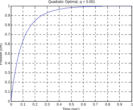
and we want to design a quadratic optimal controller with q=0.001. Show that

0

3.381 0.0169( 10)

( ) ( ) 3.5

11.832 c 8.451 p

s

G s G s G

s s f

+

= =

+ + =

s

=

for zero position error.

Simulate the system with a unit step input. Your results should look like that in Figure 1. Turn in this plot.

b) Assume we utilize the quadratic optimal algorithm as above to determine, G but rather than utilizing a prefilter, we scale the closed loop transfer function so

thatG . Show that we then get

0( )

0(0) 1

0.05916( 10) ( )

c

s G s

s +

= and G_pf =1

Simulate the system using this controller and prefilter with a unit step input. Your results should look like that in Figure 1.

Note that we are not guaranteed we will be able to get an implementable transfer function if we scale G₀( )s so that G₀(0)=1, but if we can, we get a type 1 system and there is no scaling outside the of the feedback loop (G_pf =1 )! Why do we care? See part c, d, and e below.

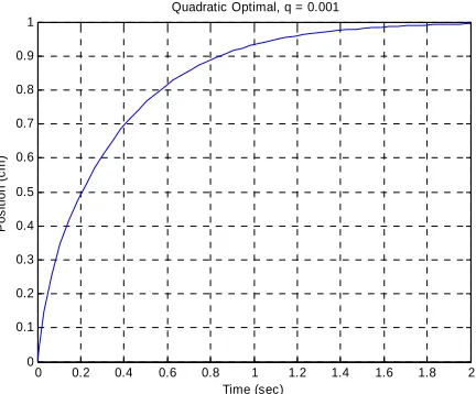
190 ( )

12 p

G s s =

+

Simulate this system with a unit step input using the controller and prefilter from part (a) using this plant instead. Your results should look like those in Figure 2.

d) Now simulate this system (plant from part c) with a unit step input using the controller and prefilter from part (b). You should get results like those in Figure 3. Turn in your graph.

e) Assume that your fool of a lab partner copied down the numbers incorrectly, and the plant is more accurately modeled as

100 ( )

20 p

G s s =

+

Show (analytically) that the position error for the original system for a step input with amplitude A is 0.68A, while the position error for the type 1 system is still 0. Simulate this plant using the original control system (part a) and the modified control system (part b). You should get results like those in Figures 4 and 5.. Turn in your graphs and your Matlab code.

5) Consider the following simple feedback system, with which we want to use model matching to determine the controller G s_c( ).

( )

G s

G s

( )

+

-However, the plant has zeros in the right half plane, and we cannot cancel these poles or we will have an unstable controller. Let's denote the plant

( ) p G s

( ) ( ) ( )

( )

L R

p

N s N s G s

D s =

where we have partitioned the numerator polynomial of the plant into which contains the zeros of the plant in the open left half plane, and which contains the zeros of the plant in the closed right half plane. Let's assume then that the desired closed loop transfer function is written as

( ) L N s

( ) R N s

( ) ( ) ( )

( )

( ) ( )

o oo R

o

o o

N s N s N s

G s

D s D s

= =

a) Show that the controller for this system is given by

( ) ( ) ( )

( )[ ( ) ( ) ( )] oo

c

L o oo R

N s D s G s

N s D s N s N s =

−

b) Insert the expression for the plant and the expression for the controller from part (a) into the block diagram, cancel where appropriate, and show by simplifying the block diagram that

( ) ( ) ( )

( )

oo R

o

o N s N s G s

D s =

Preparation for Lab 5.

6) In this problem we will modify the Matlab code closedloop_driver.m to determine the quadratic optimal controller for a given plant and value of penalty q. You should comment out those parts of the code with are not being used, do not delete them since they will be utilized later!

a) Download the file solve_quadratic.m from the class website. The input arguments to this function are (1) the transfer function of the plant Gp, and (2) the value of q. The routine returns the optimal closed loop transfer function Go(s). To use this function, in closedloop_driver.m type something like

q = 0.001;

Go = solve_quadratic(Gp,q);

Be sure all of your files are in the same directory!

b) Modify closedloop_driver.m to verify the results from problem 4a. Turn in a plot for the unit step response. Be sure to use the command minreal when manipulating transfer functions, such as finding Gc or finding the new closed loop transfer function to determine Gpre.

c) Modify closedloop_driver.m to verify the result of problem 4b (we are just looking to get the correct controller here). This should be done automatically, you should not hard code any numbers. Look at your results from Lab 1 for determining the prefilter gain.

d) Modify closedloop_driver.m to verify the results of problems 4c,d, and e. You should put in the ``new plant'' just before the simulation so it doesn't change anything else. Turn in your plots and your Malab code.

0 0.1 0.2 0.3 0.4 0.5 0.6 0.7 0.8 0.9 1 0

0.1 0.2 0.3 0.4 0.5 0.6 0.7 0.8 0.9 1

Time (sec)

P

o

s

iti

o

n

(

c

m

)

Quadratic Optimal, q = 0.001

Figure1. The step response for the correct plant and original controller (Problem 4, part a)

0 0.1 0.2 0.3 0.4 0.5 0.6 0.7 0.8 0.9 1 0

0.1 0.2 0.3 0.4 0.5 0.6 0.7 0.8 0.9

Time (sec)

P

o

s

iti

o

n

(

c

m

)

Quadratic Optimal, q = 0.001

Figure 2. The step response for the new plant and the original controller (Problem 4, part c)

0 0.1 0.2 0.3 0.4 0.5 0.6 0.7 0.8 0.9 1 0

0.1 0.2 0.3 0.4 0.5 0.6 0.7 0.8 0.9 1

Time (sec)

P

o

s

iti

o

n

(

c

m

)

Quadratic Optimal, q = 0.001

0 0.1 0.2 0.3 0.4 0.5 0.6 0.7 0.8 0.9 1 0

0.05 0.1 0.15 0.2 0.25 0.3 0.35

Time (sec)

P

o

s

iti

o

n

(

c

m

)

Quadratic Optimal, q = 0.001

Figure 4. Step response of the new plant with the original controller (Problem 4, part e)

0 0.2 0.4 0.6 0.8 1 1.2 1.4 1.6 1.8 2 0

0.1 0.2 0.3 0.4 0.5 0.6 0.7 0.8 0.9 1

Time (sec)

Po

s

iti

o

n

(

c

m

)

Quadratic Optimal, q = 0.001