Augmented Mixture Models for Lexical Disambiguation

Augmented Mixture Models for Lexical Disambiguation

Silviu Cucerzan and David Yarowsky

Department of Computer Science and Center for Language and Speech Processing

Johns Hopkins University Baltimore, MD 21218, USA {silviu,yarowsky}@cs.jhu.edu

Abstract

This paper investigates several augmented mixture models that are competitive alternatives to standard Bayesian models and prove to be very suitable to word sense disambiguation and related classifica-tion tasks. We present a new classificaclassifica-tion correc-tion technique that successfully addresses the prob-lem of under-estimation of infrequent classes in the training data. We show that the mixture models are boosting-friendly and that both Adaboost and our original correction technique can improve the re-sults of the raw model significantly, achieving state-of-the-art performance on several standard test sets in four languages. With substantially different out-put to Naïve Bayes and other statistical methods, the investigated models are also shown to be effective participants in classifier combination.

1 Introduction

The focus tasks of this paper are two re-lated problems in lexical ambiguity resolution: Word Sense Disambiguation (WSD) and Context-Sensitive Spelling Correction (CSSC).

Word Sense Disambiguation has a long history as a computational task (Kelly and Stone, 1975), and the field has recently supported large-scale interna-tional system evaluation exercises in multiple lan-guages (SENSEVAL-1, Kilgarriff and Palmer (2000), and SENSEVAL-2, Edmonds and Cotton (2001)).

General purpose Spelling Correction is also a long-standing task (e.g. McIlroy, 1982), tradi-tionally focusing on resolving typographical errors such as transposition and deletion to find the clos-est “valid” word (in a dictionary or a morpholog-ical variant), typmorpholog-ically ignoring context. Yet Ku-kich (1992) observed that about 25-50% of the spelling errors found in modern documents are ei-ther context-inappropriate misuses or substitutions of valid words (such as principal and principle) which are not detected by traditional spelling

cor-rectors. Previous work has addressed the problem of CSSC from a machine learning perspective, in-cluding Bayesian and Decision List models (Gold-ing, 1995), Winnow (Golding and Roth, 1996) and Transformation-Based Learning (Mangu and Brill, 1997).

Generally, both tasks involve the selection be-tween a relatively small set of alternatives per key-word (e.g. sense id’s such as church/BUILDING and church/INSTITUTION or commonly confused spellings such as quiet and quite), and are dependent on local and long-distance collocational and syntac-tic patterns to resolve between the set of alterna-tives. Thus both tasks can share a common feature space, data representation and algorithm infrastruc-ture. We present a framework of doing so, while in-vestigating the use of mixture models in conjunction with a new error-correction technique as competi-tive alternacompeti-tives to Bayesian models. While several authors have observed the fundamental similarities between CSSC and WSD (e.g. Berleant, 1995 and Roth, 1998), to our knowledge no previous com-parative empirical study has tackled these two prob-lems in a single unified framework.

2 Problem Formulation. Feature Space The problem of lexical disambiguation can be mod-eled as a classification task, in which each in-stance of the word to be disambiguated (target word, henceforth), identified by its context, has to be la-beled with one of the established sense labels

.1 The approaches we investigate are statistical methods

!

, out-putting conditional probability distributions over the sense set given a context "$#% . The

classifica-tion of a context " is generally made by choosing &(')+*,&.-0/2143

657" 98

, but we also present an

alterna-1

In the case of spelling correction, the classification labels are represented by the confusion set rather than sense labels (for example:<;>=@?BAC2DFE7?GAHD(I ).

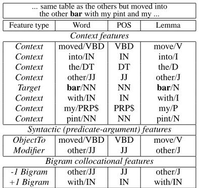
... same table as the others but moved into the other bar with my pint and my ... Feature type Word POS Lemma

Context features

Context moved/VBD VBD move/V

Context into/IN IN into/I

Context the/DT DT the/D

Context other/JJ JJ other/J

Target bar/NN NN bar/N

Context with/IN IN with/I

Context my/PRP$ PRP$ my/P

Context pint/NN NN pint/N

Syntactic (predicate-argument) features ObjectTo moved/VBD VBD move/V

Modifier other/JJ JJ other/J

Bigram collocational features -1 Bigram other/JJ JJ other/J

+1 Bigram with/IN IN with/IN Figure 1: Example context for WSD SENSEVAL-2 target word bar (inventory of 21 senses) and extracted features

tive approach in Section 4.1.

The contexts are represented as a collection

of features. Previous work in WSD and CSSC (Golding, 1995; Bruce et al., 1996; Yarowsky, 1996; Golding and Roth, 1996; Pedersen, 1998) has found diverse feature types to be useful, in-cluding inflected words, lemmas and part-of-speech (POS) in a variety of collocational and syntactic re-lationships, including local bigrams and trigrams, predicate-argument relationships, and wide-context bag-of-words associations. Examples of the feature types we employ are illustrated in Figures 1 and 2.

The syntactic features are intended to capture the predicate-argument relationships in the syn-tactic window in which the target word occurs. Different relations are considered depending on the target word’s POS. For nouns, these relations are: verb-object, subject-verb, modifier-noun, and noun-modified_noun; for verbs: object, verb-particle/preposition, verb-prepositional_object; for adjectives: modifying_adjective-noun. Also, words with the same POS as the target word that are linked to the target word by coordinating conjunctions are extracted as sibling features. The extraction pro-cess is performed using simple heuristic patterns and regular expressions over the POS environment. As Figure 2 shows, we considered for the CSSC task the POS bigrams of the immediate left and right word pairs as additional features in order to solve POS ambiguity and capture more of the syntactic environment in which the target word occurs (the elements of a confusion set often have disjoint or very different syntactic functions).

... presents another {piece,peace} of the problem ... Feature type Word POS Lemma

Context features

Context presents VBZ present/V

Context another DT another/D

Target {peace,piece} NN J /N

Context of IN of/I

Context the DT the/D

Context problem NN problem/N

Syntactic (predicate-argument) features ObjectTo presents VBZ present/V

Modifier problem NN problem/N

Bigram collocational features

-1 Bigram another DT another/D

+1 Bigram of IN of/I

Bigram POS environment

POS-2-1 - VBZ+DT

-POS+1+2 - IN+DT

-Figure 2: Example context for the spelling confusion set {piece,peace} and extracted features

3 Mixture Models (MM)

We investigate in this Section a direct statistical model that uses the same starting point as the algo-rithm presented in Walker (1987). We then compare the functionality and the performance of this model to those of the widely used Naïve Bayes model for the WSD task (Gale et al., 1992; Mooney, 1996; Pedersen, 1998), enhanced with the full richer fea-ture space beyond the traditional unordered bag-of-words.

Algorithm 1 Naïve Bayes Model

K

5

+L

"

8

K

5

98NM

K

57" L98

K

57"

8 O

(1)

K

5

98NMPRQ

1SUTWVYX

K

57Z L98

[

/]\^13

K

5

_B8NMPRQ

1SUT`VYX

K

57Z

L_B8 (2)

It is known that Bayes decision rule is optimal if the distribution of the data of each class is known (Duda and Hart, 1973, ch. 2). However, the class-conditional distributions of the data are not known and have to be estimated. Both Naïve Bayes and the mixture model we investigated estimate K

5

+L

"

8

redun-dancy of the features in the case of WSD-related tasks, in conjunction with the limited training data on which the probabilities are estimated and the high dimensionality of the feature space, these as-sumptions lead to substantial modeling problems. Another important observation is that very many of the frequencies involved in the probability esti-mation are zero because of the very sparse feature space. Naïve Bayes depends heavily on probabil-ities not being zero and therefore it has to rely on smoothing. On the other hand, the mixture model is more robust to unseen events, without the need for explicit smoothing.

Under the proposed mixture model, the condi-tional probability of a sense

given a target word

-in a context" is estimated as a mixture of the

condi-tional sense probability distributions for individual context features:

Algorithm 2 Mixture Model

K 5 +L " 8 a Q 1SUT`VYX K 5 +L Z " 8UM K 57Z L " 8 O (3) a Q 1SUT`VYX K 5 +L Z 8UM K 57Z L " 8 (4)

as opposed to the Naïve Bayes model in which the probability of a sense

given a context " is derived

from the prior probability of

weighted by the con-ditional probabilities of the contextual featuresbc57"

8

given the sense. The probabilitiesK

5

+L

Z

8

in (4) andK 57Z

L98

in (2) can be computed as maximum likelihood estimates (MLE), by counting the co-occurrences of

andZ

versus the occurrences of Z , respectively

in the training data. An extension to this classical estima-tion method is to use distance-weighted counts in-stead of raw counts for the relative frequencies:

K 5 (L Z 8 edcf '4gh 57Z ji0k9l / 8 dcf '4gh 57Z ji k 8

[ Vnm@1oprq m d 57Z " / 8 [ V21o p d 57Z " 8 (5) K 57Z L98 dcf '4gh 57Z jisk9l / 8 [tQ \1SUTWVuX dcf '4gh 57Z _vjisk9l / 8 (6) i k

denotes the training contexts of word

-and

isk9l

/

the subset of

i

k

corresponding to sense

. When

Z is a syntactic headword,

d

57Z

"

8

is computed by raw count. When Z is a context word,

d 57Z " 8 is computed as a function of the positionw of the target

word

-in" and the positionsx

x

whereZ

oc-curs in" :

d 57Z " 8 [ yWz 0{ 57w x y 8

. If{ 57w x y 8 are set to

regardless of the distance

L

ws|}x

L

then MLE es-timates are obtained. There are various other ways of choosing the weighting measure {

. One natural way is to transform the distance

L

w+|~x

y

L

into a close-ness measure by considering {

57w x y 8 j l€B.‚nƒGl

(Manning and Schütze, 1999, ch. 14.1). This mea-sure proves to be effective for the spelling correc-tion task, where the words in the immediate vicinity are far more important than the rest of the context words2, but imposes counterproductive differences between the much wider context positions (such as +30 vs. +31) used in WSD, especially when con-sidering large context windows. Experimental re-sults indicate that it is more effective to level out the local positional differences given by a continu-ous weighting, by instead using weight-equivalent regions which can be described with a simple step-function{ 5„x 2…†8 jˆ‡r‰ qŠ@‹ŒBq Ž

, ( is a constant

3_).

A filtering process based on the overall impor-tance of a word Z for the disambiguation of

-is also employed, using alterations of the form

‘“’”u•u– T Q˜— oprq m X ‘™’r”j•Y– T Qš— o p X 0›9œž p

, with Ÿ Qš—

k

proportional to the number of senses of target word

-which it co-occurs with in the training set.4 In this way, the words that occur only once in the training set, as well as those that occur with most of the senses of a word, providing no relevant information about the sense itself, are penalized.

Improvements obtained using weighted frequen-cies and filtering over MLE are shown in Table 1.

Bayes Mixture

MLE bag-of-words only 55.55 56.31

MLE with syntactic features 61.62 62.27

+ Weighting + Filtering 63.28 63.06

+ Collocational Senses5 _{65.70 65.41}

Table 1:The increase in performance for successive variants of Bayes and Mixture Model as evaluated by 5-fold cross vali-dation on SENSEVAL-2 English data

K

57Z

L

"

8

can be seen as weighting factors in the mixture model formula (4). When Z is a word,

2

Golding and Schabes (1996) show that the most important words for CSSC are contained within a window of “¡ .

3

The results shown were obtained for ¢£;¥¤ with term

weights doubled within a  “¡ context window. Various

other functions and parameters values were tried on held-out parameter-optimization data for SENSEVAL-2.

4

A normalization step is required to output probability dis-tributions.

5

K

57Z " expresses the positional relationship

be-tween the occurrences of Z and the target word

-in " , and is computed using step-functions as

de-scribed previously. When Z is a syntactic

head-word,

K

57Z

L

"

8

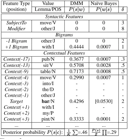
is chosen as the average value of two ratios expressing the usefulness of the headword type for the given target word and respectively for the POS-class of the target word (adjective, noun, verb). These ratios are estimated by using a jack-knife (hold-one-out) procedure on the training set and counting the number times the headword type is a good predictor versus the number of times it is a bad predictor.

Feature Type Value DMM Naïve Bayes

(position) Lemma/POS ¦¨§^©ª«“¬ ¦¨§«­ª© ¬ ®

Syntactic Features

SubjectTo move/V 0 0 3

Modifier other/J 0 0 8

Bigrams

-1 Bigram other/J 0 0 2

+1 Bigram with/I 0.4444 0.0007 1

Contextual Features

Context(-17) pub/N 0.3677 0.0007 .3

Context(-13) sit/V 0.5708 0.0028 .5

Context(-9) table/N 0.7173 0.0008 .5

Context(-4) move/V 0.2990 0.0007 1

Context(-3) into/I - -

-Context(-2) the/D - -

-Context(-1) other/J - -

-Target bar/N 0.4296 [0.0530] 2

Context(+1) with/I - -

-Context(+2) my/P - -

-Context(+3) pint/N 0.3333 0.0001 2

... ... ... ...

Posterior probability¦¨§^©ª¯2¬: ° ±³² =.46

´¶µ mG·

¸º¹ =.29

Figure 3: A WSD example that shows the influence of syntactic, collocational and long-distance context features, the probability estimates used by Naïve Bayes and MM and their associated weights (® ), and the posterior probabilities of the

true sense as computed by the two models.

As shown in Table 1, Bayes and mixture models yield comparable results for the given task. How-ever, they capture the properties of the feature space in distinct ways (example applications of the two models on the sentence in Figure 1 are illustrated in Figure 3) and therefore, are very appropriate to be used together in combination (see Section 5.4).

4 Classification Correction and Boosting We first present an original classification correction method based on the variation of posterior probabil-ity estimates across data and then the adaptation of the Adaboost method (Freund and Schapire, 1997) to the task of lexical classification.

4.1 The Maximum Variance Correction Method (MVC)

One problem arising from the sparseness of training data is that mixture models tend to excessively fa-vor the best represented senses in the training set. A probable cause is that spurious words, which can not be considered general stopwords but do not carry sense-disambiguation information for a particular target word, may occur only by chance both in train-ing and test data.6 Another cause is the fact that mixture models search for decision surfaces linear in the feature space7; therefore, they can not make only correct classifications (unless the feature space can be divided by linear conditions) and the sam-ples for the under-represented senses are likely to be interpreted as outliers.

To address this estimation problem, a second classification step is employed, based on the obser-vation that the deviation of a component of the pos-terior distribution from its expected value (as com-puted over the training set) can be as relevant as the maximum of the distribution *,&.-0/2143¨»

K

5

(L

"

8

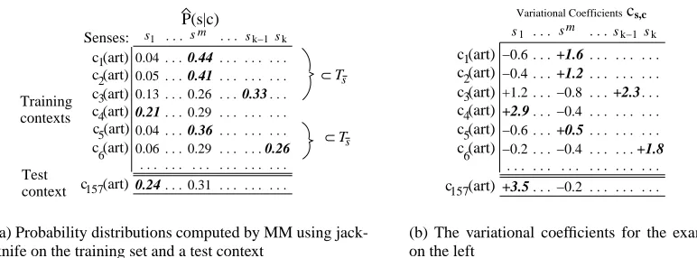
. In-stead of classifying each test context independently after estimating its sense probability distribution, we classify it by comparing it with the whole space of training contexts, for which the posterior distri-butions are computed using a jackknife procedure.

Figure 4(a) illustrates such an example: each line in the table represents the posterior distribution over senses given a context, each column contains the values corresponding to a particular sense in the posterior distributions of all contexts. Intuitively, sense

may be preferred to the most likely sense

¼

for the test context" u½@¾

5

&.' …†8

despite the fact that the »

K

5

L

"

u½@¾ 8

is smaller than »

K

5

¼<L

"

u½@¾ 8

because of the analogy with"!¿95

&(' … 8

and the “expected val-ues” of the components corresponding to

and

¼

. Unfortunately, we face again the problem of under-representation in the training data: the ex-pected values in the posterior distributions for the under-represented senses when they express the cor-rect classification can not be accurately estimated. Therefore, we have to look at the problem from an-other angle.

6

For example, assuming that every context contains approx-imately the same number of such words, then given two senses, one represented in the training set by 20 examples, and the other one by 4, it is five times more likely that a spurious word in a test context co-occurs with the larger sampled sense.

7

T_s À Ts À Test context . . . . . . . . . . . . . . . . . . . . . . . . . . . . . . . . . . . . . . s . . . . . . . . . . . . . . . . . . . . . . . . . . . . . . . . . . . . . . . . . . . . . . . . . 0.04 0.05 0.13 0.21 0.04 0.06 0.24 0.44 0.41 0.26 0.33 0.29 0.36 0.29 0.26 0.31 Training contexts 157 6 4 3 2 1

c (art) c (art) c (art) c (art) P(s|c) . . . . Senses: c (art) c (art) c (art)₅

1 sm sk−1sk

(a) Probability distributions computed by MM using jack-knife on the training set and a test context

s . . 1 2 3 4 5 6 157 c (art) c (art) c (art) c (art) c (art) c (art) c (art)

−0.2 −0.6 −0.4 −0.4 −0.2 −0.8 . . . . . . . . . . . . . . . . . . +1.6 +1.2 . . . . . . . . . . . . . . . . . . +0.5 s +3.5 . . . . . . . . . . . . . . . . . . . . . . . . . . . . . . . . . . . . . . . . . . . . . . . . . −0.4 −0.6 +1.2 +2.9 +2.3 +1.8

. . . s . . . s Variational Coefficientscs,c

1 m k−1 k

(b) The variational coefficients for the example on the left

Figure 4: WSD example showing the utility of the MVC method. A sense©

°

with a high variational coefficient is preferred to the mode©2Á of the MM distribution (the fields corresponding to the true sense are highlighted)

The mathematical support is provided by Cheby-shev’s inequality K

5 L |Äà L™Å ŸUÆ 8<Ç ›žÈ , which allows us to place an upper bound on the probabil-ity that the value of a random variable

Â

is larger than a set value, given the meanà and varianceÆ of

Â

. Considering a finite selection

i 5 -€ 8 € from a distribution É for which à andÆ exist and can be

estimated8as the empirical mean»

à l o l [ kÊ 1o -€

and empirical variance»

Æ l o l [ kÊ 1o 5 -€ | » à 8 , and given another set Ë

57Ì4Í

8

Í , the elements of

Ë that are least probable as being generated from

É are those for which the variational coefficients

Î "rÍ ÐÏ@ ÒÑ Ó ÑÔ are large.

To apply this assumption to the disambiguation task, a set

i

/

containing the values »

K 5 (L " 8 for all contexts " in the training set that are not labeled

is built for every sense

(see Figure 4(a)). In this way, the problem of poor representation of some senses is overcome and the selections

i

/

are large for all senses. An instance in the test set is consid-ered more likely to correspond to a sense

if the estimated value »

K

5

+L

"

8

is an outlier with respect to

i

/

(see Figure 4(b)) and thus it is viewed as a can-didate for having its classification changed to

. Assuming that the selections

i

/

are representa-tive and there exist first and second order moments for the underlying distributions (conditions which we call “good statistical properties”), an improve-ment in the accuracy

|ÖÕ of the classifier can

be expected when choosing a sense with a varia-tional coefficient Î

"Ä×

‰

ÒØ

instead of the

clas-sifier distribution’s mode &(')(*,&.-0/»

K 5 +L " 8 (if such a sense exists). For example, knowing that the per-formance of the mixture model for SENSEVAL-2 is

8_{It is hard to judge how well estimated these statistics are}

without making any distributional assumptions.

approximatively

ÚÙ4Û

, the threshold for variational coefficients is set to

ÚÙ4Ü

. Because spurious words not only favor the better represented senses in the training set, but also can affect the variational coef-ficients of unlikely senses, some restrictions had to be imposed in our implementation to avoid the other extreme of favoring unlikely senses.

The mixture model does not guarantee the re-quirements imposed by the MVC method are met, but it has the advantage over the Bayesian model that each of the components of the posterior distri-bution it computes can be seen as a weighted mix-ture of random variables corresponding to the indi-vidual features. In the simplest case, when consid-ering binary features, these variables are Bernoulli trials. Furthermore, if the trials have the same probability-mass function then a component of the posterior distribution will follow a binomial distri-bution, and therefore would have good statistical properties. In general, the underlying distributions can not be computed, but our experiments show that they usually have good statistical properties as re-quired by MVC.

4.2 AdaBoost

AdaBoost is an iterative boosting algorithm intro-duced by Freund and Schapire (1997) shown to be successful for several natural language classifica-tion tasks. AdaBoost successively builds classifiers based on a weak learner (base learning algorithm) by weighting differently the examples in the training space, and outputs the final classification by mix-ing the predictions of the iteratively built classifiers. Because sense disambiguation is a multi-class prob-lem, we chose to use version AdaBoost.M2.

fea-ture space. Superficial modeling of the training set can easily be achieved because of the singu-larity/rarity of many feature values in the context space, but this largely represents overfitting of the training data. In order to solve this problem, we use AdaBoost in conjunction with jackknife and a partial updating technique. At each round,Ý

clas-sifiers are built using as training all the examples in the training set except the one to be classified, and the weights are updated at feature level rather than context level. This modified Adaboost algorithm could only be implemented for the mixture model, which “perceives” the contexts as additive mixture of features. The Adaboost-enhanced mixture model is called AdaMixt henceforth.

5 Evaluation

We present a comparative study for four languages (English, Swedish, Spanish, and Basque) by per-forming 5-fold cross-validation on the SENSEVAL-2 lexical-sample training data, using the fine-grained sense inventory. For English and Swedish, for which POS-tagged training data was available to us, the fnTBL algorithm (Ngai and Florian, 2001) based on Brill (1995) was used to annotate the data, while for Spanish a mildly-supervised POS-tagging system similar to the one presented in Cucerzan and Yarowsky (2000) was employed. We also present the results obtained by the different algorithms on another WSD standard set, SENSEVAL-1, also by performing 5-fold cross validation on the original training data. For CSSC, we tested our system on the identical data from the Brown corpus used by Golding (1995), Golding and Roth (1996) and Mangu and Brill (1997). Finally, we present the re-sults obtained by the investigated methods on a sin-gle run on the Senseval-1 and Senseval-2 test data.

The described models were initially trained and tested by performing 5-fold cross-validation on the

SENSEVAL-2 English lexical-sample-task training

data. When parameters needed to be estimated, jackknife or a 3-1-1 split (training and/or parame-ter estimation - testing) were used.

5.1 SENSEVAL-2

The English training set for SENSEVAL-2 is com-posed of 8861 instances representing 73 target words with an average number of 12.5 senses per word. Table 2 illustrates the performance of each of the studied models broken down by part-of-speech. As observed in most experiments, the feature-enhanced Naïve Bayes has the tendency

to outperform by a small margin the raw mixture model, but because the latter proved to be boosting-friendly, its augmented versions achieved the high-est final accuracies. The difference between MMVC and enhanced Naïve Bayes is significant (McNemar rejection risk ofÞ~

ß

).

Adjectives Nouns Verbs Overall

Most Likely 52.11 52.01 27.28 41.79

Naïve Bayes (FE) 73.18 72.74 55.54 65.70

Mixture 73.90 71.09 56.16 65.41

AdaMixt 74.68 72.17 56.41 66.09

MMVC 74.68 73.06 57.06 66.72

Table 2:Results using 5-fold cross validation on SENSEVAL -2 English lexical-sample training data

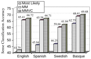
Figure 5 shows both the performance of the mix-ture model alone and in conjunction with MVC, and highlights the improvement in performance achieved by the latter for each of the 4 languages. All MMVC versus MM differences are statistically significant (for SENSEVAL-2 English data, the rejec-tion probability of a paired McNemar test is

 uà ). 40 45 50 55 60 65 70 75

English Spanish Swedish Basque Most Likely MM MMVC ááá ááá ááá ááá ââ ââ ââ ââ ãã ãã ãã ää ää ää åå åå åå åå åå åå åå åå åå åå åå åå åå åå åå åå åå åå åå åå åå åå åå åå ææ ææ ææ ææ ææ ææ ææ ææ ææ ææ ææ ææ ææ ææ ææ ææ ææ ææ ææ ææ ææ ææ ææ çç çç çç çç çç çç çç çç çç çç çç çç çç çç çç çç çç çç çç çç çç çç çç çç èè èè èè èè èè èè èè èè èè èè èè èè èè èè èè èè èè èè èè èè èè èè èè éé éé êê êê ëë ëë ëë ëë ëë ëë ëë ëë ëë ëë ìì ìì ìì ìì ìì ìì ìì ìì ìì ìì íí íí íí íí íí íí íí íí íí íí íí íí íí íí íí íí íí íí íí îî îî îî îî îî îî îî îî îî îî îî îî îî îî îî îî îî îî îî ïïï ïïï ïïï ïïï ïïï ïïï ïïï ïïï ïïï ïïï ïïï ïïï ïïï ïïï ïïï ïïï ïïï ïïï ïïï ïïï ïïï ïïï ïïï ïïï ïïï ððð ððð ððð ððð ððð ððð ððð ððð ððð ððð ððð ððð ððð ððð ððð ððð ððð ððð ððð ððð ððð ððð ððð ððð ððð ñ ò ó ó ó ô ô

Sense Classification Accuracy

45.94 46.25 65.58 68.61 61.84 59.66 62.75 69.68 66.71 41.79 66.72 65.41

Figure 5: MM and MMVC performance by performing 5-fold cross validation on SENSEVAL-2 data for 4 languages

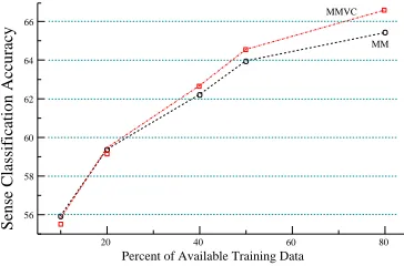
Figure 6 shows what is generally a log-linear in-crease in performance of MM alone and in combi-nation with the MVC method over increasing train-ing sizes. Because of the way the smallest traintrain-ing sets were created to include at least one example for each sense, they were more balanced as a side effect, and the compensations introduced by MVC were less productive as a result. Given more training data, MMVC starts to improve relative to the raw model both because the training sets become more unbal-anced in their sense distributions and because the empirical moments and the variational coefficients on which the method relies are better estimated.

5.2 SENSEVAL-1

20 40 60 80 Percent of Available Training Data

56 58 60 62 64 66

Sense Classification Accuracy

MMVC

MM

Figure 6: Learning Curve for MM and MMVC on SENSEVAL-2 English (cross-validated on heldout data)

data (30 words, 12479 instances, with an average of 10.8 senses per word) by using 5-fold cross val-idation. There was no further tuning of the feature space or model parameters to adapt them to the par-ticularities of this new test set. Comparative perfor-mance is shown in Table 3. The difference between MMVC and enhanced Naïve Bayes is statistically significant (McNemar rejection risk 0.036).

Adjectives Nouns Verbs Overall

Most Likely 63.43 66.52 57.6 63.09

Naïve Bayes (FE) 75.67 84.15 76.65 80.16

Mixture 76.45 81.57 75.9 78.79

AdaMixt 76.83 83.39 77.10 80.16

MMVC 78.49 84.79 76.81 81.06

Table 3:Results using 5-fold cross validation on SENSEVAL -1 training data (English)

5.3 Spelling Correction

Both MM and the enhanced Bayes model obtain vir-tually the same overall performance9 as the TriB-ayes system reported in (Golding and Schabes, 1996), which uses a similar feature space. The correction and boosting methods we investigated marginally improve the performance of the mixture model, as can be seen in Table 4 but they do not achieve the performance of RuleS 93.1% (Mangu and Brill, 1997) and Winnow 93.5% (Golding and Roth, 1996; Golding and Roth, 1999), methods that include features more directly specialized for spelling correction. Because of the small size of the test set, the differences in performance are due to only 14 and 20 more incorrectly classified exam-ples respectively. More important than this differ-ence10 may be the fact that the systems built for WSD were able to achieve competitive performance

9_{All figures reported are for the standard 14 confusion sets;}

the accuracies for the 18 sets are generally higher.

10_{We did not have the actual classifications from the other}

systems to check the significance of the difference.

with little to no adaptation (we only enriched the feature space by adding the POS bigrams to the left and right of the target word and changed the weight-ing model as presented in Section 3 because spellweight-ing correction relies more on the immediate than long-distance context). Another important aspect that can

test

size M.L. Bayes MM AdaMixt MMVC

accept 50 70.0 92.0 90.0 90.0 94.2

affect 49 91.8 95.9 98.0 98.0 93.9

among 186 71.5 80.6 78.5 81.2 80.6

amount 123 71.5 79.7 79.7 82.9 83.7

begin 146 93.2 96.6 96.6 97.3 96.6

country 62 91.9 93.5 95.2 93.5 93.5

lead 49 46.9 93.9 91.8 95.9 91.8

past 74 68.9 86.5 93.2 93.2 93.2

peace 50 44.0 78.0 80.0 78.0 80.0

principal 34 58.8 82.3 88.2 85.3 88.2

quiet 66 83.3 93.9 93.9 93.9 95.5

raise 39 64.1 87.2 84.6 84.6 87.2

than 514 63.4 96.9 96.5 96.5 96.5

weather 61 86.9 98.4 95.1 96.7 98.4

Overall 1503 71.1 91.2 91.2 91.8 92.2

Table 4:Results on the standard 14 CSSC data sets be seen in Table 4 is that there was no model that constantly performed best in all situations, suggest-ing the advantage of developsuggest-ing a diverse space of models for classifier combination.

5.4 Using MMVC in Classifier Combination

The investigated MMVC model proves to be a very effective participant in classifier combination, with substantially different output to Naïve Bayes (9.6% averaged complementary rate, as defined in Brill and Wu (1998)). Table 5 shows the im-provement obtained by adding the MMVC model to empirically the best voting system we had us-ing Bayes, BayesRatio, TBL and Decision Lists (all classifier combination methods tried and their results are presented exhaustively in Florian and Yarowsky (2002)). The improvement is significant in both cases, as measured by a paired McNemar test:

Wõ



¾

for SENSEVAL-1 data,

Úö



¾

for SENSEVAL-2 data. without

MMVC MMVCwith reductionerror

Senseval1 82.26 83.06 4.5%

Senseval2 67.53 68.66 3.5%

Table 5: The contribution of MMVC in a rank-based classi-fier combination on SENSEVAL-1 and SENSEVAL-2 English as computed by 5-fold cross validation over training data

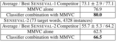
data, with an accuracy of 62.5%. Table 6 contrasts the performance obtained by the MMVC method to the average and best system performance in the two

SENSEVAL exercises.

SENSEVAL-1 (30 target words, 7446 instances)

Average / Best SENSEVAL-1 Competitor 73.1  2.9 / 77.1

MMVC alone 76.9

Classifier combination with MMVC 80.0

SENSEVAL-2 (73 target words, 4328 instances)

Average / Best SENSEVAL-2 Competitor 55.7  5.3 / 64.2

MMVC alone 62.5

Classifier combination with MMVC 66.5

Table 6: Accuracy on SENSEVAL-1 and SENSEVAL-2 En-glish test data (only the supervised systems with a coverage of at least 97% were used to compute the mean and variance)

6 Conclusion

We investigated the properties and performance of mixture models and two augmenting methods in an unified framework for Word Sense Disambiguation and Context-Sensitive Spelling Correction, showing experimentally that such joint models can success-fully match and exceed the performance of feature-enhanced Bayesian models. The new classifica-tion correcclassifica-tion method (MVC) we propose suc-cessfully addresses the problem of under-estimation of less likely classes, consistently and significantly improving the performance of the main mixture model across all tasks and languages. Finally, since the mixture model and its improvements performed well on two major tasks and several multilingual data sets, we believe that they can be productively applied to other related high-dimensionality lexi-cal classification problems, including named-entity classification, topic classification, and lexical choice in machine translation.

References

D. Berleant. 1995. Engineering "word experts" for word disam-biguation. Natural Language Engineering, 1(4):339–362. E. Brill and J. Wu. 1998. Classifier combination for improved

lexical disambiguation. In Proceedings of COLING-ACL’98, pages 191–195.

E. Brill. 1995. Transformation-based error-driven learning and natural language processing: A case study in part of speech tagging. Computational Linguistics, 21(4):543–565. R. Bruce, J. Wiebe, and T. Pedersen. 1996. The measure of a

model. In Proceedings of EMNLP-1996, pages 101–112. S. Cucerzan and D. Yarowsky. 2000. Language independent

minimally supervised induction of lexical probabilities. In

Proceedings of ACL-2000, pages 270–277.

R. O. Duda and P. E. Hart. 1973. Pattern Classification and

Scene Analysis. Wiley.

P. Edmonds and S. Cotton. 2001. SENSEVAL-2 overview. In

Proceedings of SENSEVAL-2, pages 1–6.

R. Florian and D. Yarowsky. 2002. Modeling consensus: Classi-fier combination for word sense disambiguation. In

Proceed-ings of EMNLP-2002.

Y. Freund and R. E. Schapire. 1997. A decision-theoretic gener-alization of on-line learning and application to boosting.

Jour-nal of Computer and System Sciences, 55:119–139.

W. Gale, K. Church, and D. Yarowsky. 1992. A method for disambiguating word senses in a large corpus. Computers and

the Humanities, 26:415–439.

A. R. Golding and D. Roth. 1996. Applying winnow to context-sensitive spelling correction. In Machine Learning:

Proceed-ings of the 13th International Conference, pages 182–190.

A. R. Golding and D. Roth. 1999. A winnow-based approach to context-sensitive spelling correction. Machine Learning, 34(1-3):107–130.

A. R. Golding and Y. Schabes. 1996. Combining trigram-based and feature-based methods for context-sensitive spelling cor-rection. In Proceedings of ACL-1996, pages 71–78.

A. R. Golding. 1995. A Bayesian hybrid method for context-sensitive spelling correction. In Proceedings of the Third

Workshop on Very Large Corpora, pages 39–53.

E. F. Kelly and P. J. Stone. 1975. Computer Recognition of

English Word Senses. North Holland Press.

A. Kilgarriff and M. Palmer. 2000. Introduction to the special issue onSENSEVAL. Computers and the Humanities, 34(1-2):1–13.

K. Kukich. 1992. Techniques for automatically correcting words in text. ACM Computing Surveys, 24(4):377–439.

L. Mangu and E. Brill. 1997. Automatic rule acquisition for spelling correction. In Proceedings of the 14th International

Conference on Machine Learning, pages 734–741.

C.D. Manning and H. Schütze. 1999. Foundations of Statistical

Natural Language Processing. MIT Press.

M. D. McIlroy. 1982. Development of a spelling list.

j-IEEE-TRANS-COMM, COM-30(1):91–99.

R. J. Mooney. 1996. Comparative experiments on disambiguat-ing word senses: An illustration of the role of bias in machine learning. In Proceedings of EMNLP-1996, pages 82–91. G. Ngai and R. Florian. 2001. Transformation-based learning in

the fast lane. In Proceedings of NAACL-2001, pages 40–47. T. Pedersen. 1998. Naïve Bayes as a satisficing model. In

Work-ing Notes of the AAAI SprWork-ing Symposium on SatisficWork-ing Mod-els, pages 60–67.

D. Roth. 1998. Learning to resolve natural language ambiguities: a unified approach. In Proceedings of the 15th Conference of

the AAAI, pages 806–813.

D. E. Walker. 1987. Knowledge resource tools for accessing large text files. In Sergei Nirenburg, editor, Machine

Trans-lation: Theoretical and Methodogical Issues, pages 247–261.

Cambridge University Press.

D. Yarowsky. 1996. Homograph disambiguation in speech

synthesis. In J. Olive J. van Santen, R. Sproat and