A Utility Model of Authors in the Scientific Community
Yanchuan Sim
School of Computer Science Carnegie Mellon University Pittsburgh, PA 15213, USA
Bryan R. Routledge
Tepper School of Business Carnegie Mellon University Pittsburgh, PA 15213, USA
Noah A. Smith
Computer Science & Engineering University of Washington
Seattle, WA 98195, USA [email protected]
Abstract
Authoring a scientific paper is a complex process involving many decisions. We in-troduce a probabilistic model of some of the important aspects of that process: that authors have individual preferences, that writing a paper requires trading off among the preferences of authors as well as ex-trinsic rewards in the form of commu-nity response to their papers, that prefer-ences (of individuals and the community) and tradeoffs vary over time. Variants of our model lead to improved predictive ac-curacy of citations given texts and texts given authors. Further, our model’s pos-terior suggests an interesting relationship between seniority and author choices.
1 Introduction
Why do we write? As researchers, we write pa-pers to report new scientific findings, but this is not the whole story. Authoring a paper involves a huge amount of decision-making that may be influenced by factors such as institutional incen-tives, attention-seeking, and pleasure derived from research on topics that excite us.
We propose that text collections and associated metadata can be analyzed to reveal optimizing be-havior by authors. Specifically, we consider the ACL Anthology Network Corpus (Radev et al., 2013), along with author and citation metadata. Our main contribution is a method that infers two kinds of quantities about an author: her associ-ations with interpretable research topics, which might correspond to relative expertise or merely to preferences among topics to write about; and a tradeoff coefficient that estimates the extent to which she writes papers that will be cited versus papers close to her preferences.
The method is based on a probabilistic model that incorporates assumptions about how authors
decide what to write, how joint decisions work when papers are coauthored, and how individual and community preferences shift over time. Cen-tral to our model is a low-dimensional topic rep-resentation shared by authors (in defining prefer-ences), papers (i.e., what they are “about”), and the community as a whole (in responding with ci-tations). This method can be used to make predic-tions; empirically, we find that:
1. topics discovered by generative models out-perform a strong text regression baseline (Yo-gatama et al., 2011) for citation count predic-tion;
2. such models do better at that taskwithout mod-eling author utility as we propose; and
3. the author utility model leads to better pre-dictive accuracy when answering the question, “given a set of authors, what are they likely to write?”
This method can also be used for exploration and to generate hypotheses. We provide an in-triguing example relating author tradeoffs to age within the research community.
2 Notation and Representations
In the following, a documentdwill be represented by a vectorθd∈RK. The dimensions of this vec-tor might correspond to elements of a vocabulary, giving a “bag of words” encoding; in this work they correspond to latent topics.
Documentdis assumed to elicit from the scien-tific community an observable responseyd, which might correspond to the number of citations (or downloads) of the paper.
Each authorais associated with a vectorηa ∈
RK, with dimensions indexed the same as docu-ments. Below, we will refer to this vector as a’s “preferences,” though it is important to remember that they could also capture an author’sexpertise,
and the model makes no attempt to distinguish be-tween them. We use “preferences” because it is a weaker theoretical commitment.
3 Author Utility Model
We describe the components of our model— author utility (§3.1), coauthorship (§3.2), topics (§3.3), and temporal dynamics (§3.4)—then give the full form in§3.5.
3.1 Modeling Utility
Our main assumption about authorais that she is an optimizer: when writing documentdshe seeks to increase the responseydwhile keeping the con-tents ofd, θd, “close” to her preferencesηa. We encode her objectives as a utility function to be maximized with respect toθd:
U(θd) =κayd−12kθd−(ηa+d,a)k22 (1)
where d,a is an author-paper-specific idiosyn-cratic randomness that is unobserved to us but as-sumed known to the author. (This is a common assumption in discrete choice models. It is often called a “random utility model.”)
Notice the tradeoff between maximizing the re-sponseydand staying close to one’s preferences. We capture these competing objectives by formu-lating the latter as a squared Euclidean distance between ηa and θd, and encoding the tradeoff between extrinsic (citation-seeking) and intrinsic (preference-satisfying) objectives as the (positive) coefficient κa. If κa is large, a might be un-derstood as a citation-maximizing agent; if κa is small, a might appear to care much more about certain kinds of papers (ηa) than about citation.
This utility function considers only two partic-ular facets of author writing behavior; it does not take into account other factors that may contribute to an author’s objective. For this reason, some care is required in interpreting quantities likeκa. For example, divergence between a particularηa and
θdmight suggest thatais open to new topics, not merely hungry for citations. Other motivations, such as reputation (notoriously difficult to mea-sure), funding maintenance, and the preferences of peer referees are not captured in this model. Sim-ilarly for preferencesηa, a large value in this vec-tor might reflecta’s skill or the preferences ofa’s sponsors rather thana’s personal interest the topic. Next, we model the response yd. We assume that responses are driven largely by topics, with
some noise, so that
yd=β>θd+ξd (2) where ξd ∼ N(0,1). Because the community’s interest in different topics varies over time, β is given temporal dynamics, discussed in§3.4.
Under this assumption, the author’s expected utility assuming she is aware of β (often called “rational expectations” in discrete choice models), is:
E[U(θd)] =κaβ>θd−21kθd−(ηa+d,a)k22 (3)
(This is obtained by plugging the expected value ofyd, from Eq. 2, into Eq. 1.)
An author’s decision will therefore be
ˆ
θd= arg max
θ κaβ
>θ−1
2kθ−(ηa+d,a)k22 (4)
Optimality implies that θˆd solves the first-order equations
κaβj−(ˆθd,j−(ηa,j +d,a,j)) = 0, ∀1≤j ≤K (5) Eq. 5 highlights the tradeoff the author faces: whenβj > 0, the author will write more onθd,j, while straying too far fromηa,j incurs a penalty. 3.2 Modeling Coauthorship
Matters become more complicated when multiple authors write a paper together. Suppose the docu-mentdis authored by set of authorsad. We model the joint expected utility ofadin writingθdas the average of the group’s utility.1
E[U(θd)] = |a1d|
X
a∈ad
κaβ>θd
−12cd,akθd−(ηa+d,a)k22
(6)
where the “cost” term is scaled bycd,a, denoting the fractional “contribution” of authorato docu-mentd. Thus,Pa∈adcd,a = 1, and we treatcdas
a latent categorical distribution to be inferred. The first-order equation becomes
X
a∈ad
κaβ−cd,a(θd−(ηa+d,a)) =0 (7)
3.3 Modeling Document Content
As noted before, there are many possible ways to represent and model document content θd. We treat θd as (an encoding of) a mixture of topics. Following considerable past work, a “topic” is de-fined as a categorical distribution over observable tokens (Blei et al., 2003; Hofmann, 1999). Letwd be the observed bag of tokens constituting docu-mentd. We assume each token is drawn from a mixture over topics:
p(wd|θd) =
X
zd
Nd Y
i=1
p(zd,i |θd)p(wd,i |φzd,i)
whereNdis the number of tokens in documentd, zd,i is the topic assignment ford’sith tokenwd,i, andφ1, . . . ,φKare topic-term distributions. Note thatθd∈RK; we definep(z|θd)as a categorical draw from the softmax-transformed θd (Blei and Lafferty, 2007).
Using topic mixtures instead of a bag of words provides us with a low-dimensional interpretable representation that is useful for analyzing authors’ behaviors and preferences. Each dimensionj of an author’s preference is grounded in topic j. If we ignore document responses, this component of model closely resembles the author-topic model (Rosen-Zvi et al., 2004), except that we assume a different prior for the topic mixtures.
3.4 Modeling Temporal Dynamics
Individual preferences shift over time, as do those of the research community. We extend our model to allow variation at different timesteps. Let t ∈ h1, . . . , Ti index timesteps (in our experiments, eacht is a calendar year). We letβ(t), η(t)
a , and κ(at)denote the community’s response coefficients, authora’s preferences, and authora’s tradeoff co-efficient at timestept.
Again, we must take care in interpreting these quantities. Do changes in community interest drive authors to adjust their preferences or exper-tise? Or do changing author preferences aggregate into community-wide shifts? Or do changes in the economy or funding availability change authors’ tradeoffs? Our model cannot differentiate among these different causal patterns. Our method is use-ful for tracking these changes, but it does not pro-vide an explanation forwhythey take place.
Modeling the temporal dynamics of a vector-valued random variable can be accomplished
us-ing a multivariate Gaussian distribution. Follow-ing Yogatama et al. (2011), we assume the prior forβ(j·) = hβj(1), . . . , βj(T)ihas a tridiagonal pre-cision matrixΛ(λ, α)∈RT×T:
Λ(λ, α) =λ
1 +α −α 0 0 . . .
−α 1 + 2α −α 0 . . .
0 −α 1 + 2α −α . . .
0 0 −α 1 + 2α . . .
... ... ... ... ...
The two hyperparametersαandλcapture, respec-tively, autocorrelation (the tendency of βj(t+1) to be similar toβ(jt)) and overall variance. This ap-proach to modeling time series allows us to cap-ture temporal dynamics while sharing statistical strength of evidence across all time steps.
We use the notationT(λ, α) ≡ N(0,Λ(λ, α))
for this multivariate Gaussian distribution, in-stances of which are used as priors over response coefficientsβ, author preferencesηa, and (trans-formed) author tradeoffslogκa.
.
Observed evidence wd,i ith token in documentd
V vocabulary size
Nd number of tokens in documentd yd response to documentd A the set of authors
ad set of authors of documentd(⊆ A) T number of timesteps
Dt the set of documents from timestept D the set of all documents(=ST
t=1Dt) Latent variables
β(t) response coefficients at timet(∈RK) ηa(t) authora’s topic preferences at timet
(∈RK)
κ(at) authora’s tradeoff coefficient at timet (∈R≥0)
θd documentdtopic associations (∈RK) cd,a authora contrtibution to documentd
(P
a∈adcd,a= 1)
φk distribution over terms for topick zd,i topic assignment ofwd,i
Constants and hyperparameters K number of topics
ρ symmetric Dirichlet hyperparameter forφk
σ2
c variance hyperparameter for author contributionscd
{λ(β), α(β)}, {λ(η), α(η)}, {λ(κ), α(κ)}
[image:3.595.307.527.394.743.2]hyperparameters for priors of β,η, andlogκrespectively
3.5 Full Model
Table 1 summarizes all of the notation. The log-likelihood of our model is:
L= logp(β) +X
d∈D
logp(cd)
+X
d∈D
logp(yd|θd,β) + logp(wd|θd)
+X
a∈A
logp(ηa) + logp(κa)
+X
d∈D
X
a∈ad
logp(θd|β,ηa, κa, cd,a) (8)
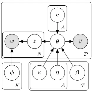
We adopt a Bayesian approach to parameter esti-mation. The generative story, including all priors, is as follows. Recall thatT(·,·)denotes the time series prior discussed in §3.4. See also the plate diagram for the graphical model in Fig. 1.
1. For each topick∈ {1, . . . , K}:
(a) Draw response coefficients β(k·) ∼ T(λ(β), α(β))and term distributionφk ∼
Dirichlet(ρ).
(b) For each author a ∈ A, draw pref-erence strengths for topic k over time, hηa,k(1), . . . , ηa,k(t)i ∼ T(λ(η), α(η)).
2. For each author a ∈ A, draw (transformed) tradeoff parameters hlogκ(1)a , . . . ,logκ(aT)i ∼ T(λ(κ), α(κ)).
3. For each timestep t ∈ {1, . . . , T}, and each documentd∈ Dt:
(a) Draw author contributions cd ∼ Softmax(N(0, σ2
cI)). This is known as a logistic normal distribution (Aitchi-son, 1986).
(b) Drawd’s topic distributions (this distribu-tion is discussed further below):
θd∼ N
X
a∈ad κ(t)
a β(t)+cd,aηa(t),kcdk22I
(9)
(c) For each token i ∈ {1, . . . , Nd}, draw topic zd,i ∼ Categorical(Softmax(θd)) and termwd,i ∼Categorical(φzd,i).
(d) Draw response yd ∼ N β(td)>θd,1; note that it collapses out ξd, which is drawn from a standard normal.
Eq. 9 captures the choice by authorsadof a dis-tribution over topics θd. Assuming that the d,as are i.i.d. and Gaussian, from Eq. 7, we get
θd=
X
a∈ad
κaβ+cd,aηa+cd,ad,a,
w z θ y
η
φ κ β
c
N
A
D
[image:4.595.84.290.96.234.2]K A T
Figure 1: Plate diagram for author utility model. Hyperparameters and edges between consecutive time steps ofβ,ηandκare omitted for clarity.
and the linear additive property of Gaussians gives us
θd∼ N
X
a∈ad
κaβ+cd,aηa,kcdk22I !
In§3.1 we described a utility function for each author. The model we are estimating is similar to those estimated in discrete choice economet-rics (McFadden, 1974). We assumed that authors are utility maximizing (optimizing) and that their optimal topic distribution satisfies the first-order conditions (Eq. 7). However, we cannot see the idiosyncratic component, d,a, which is assumed to be Gaussian; as noted, this is known as a ran-dom utility model. Together, these assumptions give the structure of the distribution over topics in terms of (estimated) utility, which allows us to naturally incorporate the utility function into our probabilistic model in a familiar way (Sim et al., 2015).
4 Learning and Inference
Exact inference in our model is intractable, so we resort to an approximate inference technique based on Monte Carlo EM (Wei and Tanner, 1990). During the E-step, we perform Bayesian inference over latent parameters (η,κ,z,θ,c,φ) using a Metropolis-Hastings within Gibbs algo-rithm (Tierney, 1994), and in the M-step, we compute maximum a posteriori estimates of β
would slow mixing of the MCMC chain.
E-step. We sample eachη(td)
a , cd,logκ(a·), and
θdblockwise using the Metropolis-Hastings algo-rithm with a multivariate Gaussian proposal distri-bution, tuning the diagonal covariance matrix to a target acceptance rate of 15-45% (see appendix§A for sampling equations).
For z, we integrate outφand sample eachzd,i directly from
p(zd,i =k|θd,φk)∝exp(θd,k)
Ck,w−d,id,i+ρ Ck,−·d,i+V ρ
where Ck,w−d,i and Ck,−·d,i are the number of times w is associated with topic k, and the number of tokens associated with topickrespectively.
We run the E-step Gibbs sampler to collect 3,500 samples, discarding the first 500 samples for burn-in and only saving samples at every third it-eration.
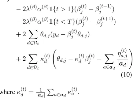
M-step. We approximate the expectations of our latent variables using the samples collected dur-ing the E-step, and directly optimizeβ(t)using
L-BFGS (Liu and Nocedal, 1989),2which requires a
gradient. The gradient of the log-likelihood with respect toβ(jt)is
∂L
∂βj(t) =−2λ
(β)β(t)
j
−2λ(β)α(β)1{t >1}(β(t)
j −βj(t−1)) −2λ(β)α(β)1{t < T}(β(t)
j −βj(t+1))
+ 2 X
d∈Dt
θd,j(yd−βj(t)θd,j)
+ 2 X
d∈Dt
κd(t) θd,j−κd(t)β(jt)−
X
a∈ad
ηa,j(t) |ad|
!
(10)
whereκ(dt)= |a1d|Pa∈adκ
(t)
a .
We ran L-BFGS until convergence3 and slice
sampled the hyperparametersλ(η), α(η), λ(κ), α(κ)
(with vague priors) at the end of the M-step. We fix the symmetric Dirichlet hyperparameter ρ = 1/V, and tunedλ(β), α(β)on a held-out
develope-ment dataset by grid search over{0.01,0.1,1,10}.
2We used libLBFGS, an open source C++ implementation (https://github.com/chokkan/liblbfgs).
3Relative tolerance of10−4.
During initialization, we randomly set the topic as-signments, while the other latent parameters are set to 0. We ran the model for 10 EM iterations. Inference. During inference, we fix the model parameters and only sample(θ,z) for each doc-ument. As in the E-step, we discard the first 500 samples, and save samples at every third iteration, until we have 500 posterior samples. In our ex-periments, we found the posterior samples to be reasonably stable after the initial burn in.
5 Experiments
Data. The ACL Anthology Network Corpus contains 21,212 papers published in the field of computational linguistics between 1965 and 2013 and written by 17,792 authors. Additionally, the corpus provides metadata such as authors, venue and in-community citation networks. For our ex-periments, we focused on conference papers pub-lished between 1980 and 2010.4We tokenized the
texts, tagged the tokens using the Stanford POS tagger (Toutanova et al., 2003), and extracted n -grams with tags that follow the simple (but effec-tive) pattern of (Adj|Noun)∗ Noun (Justeson and Katz, 1995), representing the dth document as abag of phrases (wd). Note that phrases can also be unigrams. We pruned phrases that appear in< 1%or > 95% of the documents, obtaining a vocabulary of V = 6,868 types. The pruned corpus contains 5,498 documents and 2,643,946 phrase tokens written by 5,575 authors. We let re-sponses
yd= log(1 +# of incoming citations in 3 years)
For our experiments, we used 3 different ran-dom splits of our data (70% train, 20% test, and 10% development) and averaged quantities of in-terest. Furthermore, we remove an author from a paper in the development or test set if we have not seen him before in the training data.
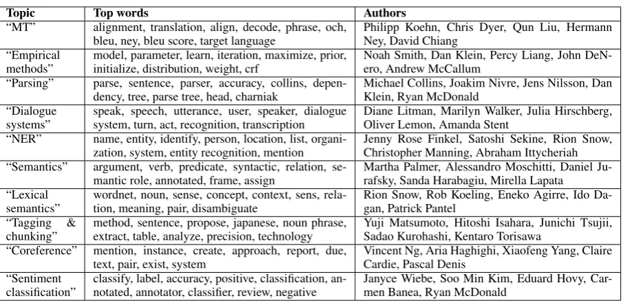
[image:5.595.74.292.484.644.2]5.1 Examples of Authors and Topics
Table 2 illustrates ten manually selected topics (out of 64) learned by the author utility model. Each topic is labeled with the top 10 words most likely to be generated conditioned on the topic
(φk). For each topic, we compute an author’s topic preference score:
TPS(a, k) =η(td)
a,k
X
d∈Da
[Softmax(θd)]k×yd
where Softmax(x) = exp(x)
P
iexp(xi). The TPS scales
the author’s η preferences by the relative num-ber of citations that the author received for the topic. This way, we can account for different
ηs over time, and reduce variance due to authors who publish less frequently.5 For each topic, the
five authors with the highest TPS are displayed in the rightmost column of Table 2. These top-ics were among the roughly one third (out of 64) that seemed to coherently map to research topics within NLP. Some others corresponded to parts of a paper (e.g., explaining notation and formulae, experiments) or to stylistic groups (e.g., “ratio-nal words” includingrather, fact, clearly, argue, clear,perhaps). Others were not interpretable to us.
5.2 Predicting Responses
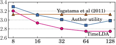
We compare against two baselines for predicting in-community citations. Yogatama et al. (2011) is a strong baseline for predicting responses; they in-corporatedn-gram features and metadata features in a generalized linear model with the time series prior discussed in§3.4.6 We also compare against
a version of our model without the author utility component. This equates to replacing Yogatama et al.’s features with LDA topic mixtures, and per-forming joint learning of the topics and citations; we therefore call it “TimeLDA.” Without the time series component, TimeLDA would instantiate su-pervised LDA (McAuliffe and Blei, 2008). Fig-ure 2 shows the mean absolute error (MAE) for the three models.
With sufficiently many topics (K ≥ 16), topic representations achieve lower error than surface features. Removing the author utility component from our model leads to better predictive perfor-mance. This is unsurprising, since our model forces β to explain both the responses (what is
5The TPS is only a measure of an author’s propensity to write papers in a specific topic area and is not meant to be a measure of an author’s reputation in a particular research sub-field.
6For the ACL dataset, Yogatama et al. (2011)’s model predicts whether a paper will receive at least 1 citation within three years, while here, we train it to predictlog(1 + #citations)instead.
8 16 32 64 128
2.6 2.8 3.0 3.2 3.4
Yogatama et al (2011)
[image:6.595.315.519.70.150.2]TimeLDA Author utility
Figure 2: Mean absolute error (in citation counts) for predicted citation counts (y-axis) against the number of topics K (x-axis). Errors are in ac-tual citation counts, while the models are trained with log counts. TimeLDA significantly outper-forms Yogatama et al. (2011) forK ≥64(paired t-test, p < 0.01), while the differences between Yogatama et al. (2011) and author utility are not significant. The MAE is calculated over 3 random splits of the data with 809, 812, and 811 docu-ments in the test set respectively.
evaluated here) and the divergence between author preferences ηa and what is actually written. The utility model is nonetheless competitive with the Yogatama et al. baseline.
5.3 Predicting Words
“Given a set of authors, what are they likely to write?” — we use perplexity as a proxy to mea-sure the content predictive ability of our model. Perplexity on a test set is commonly used to quan-tify the generalization ability of probabilistic mod-els and make comparisons among modmod-els over the same observation space. For a documentwd writ-ten by authorsad, perplexity is defined as
perplexity(wd|ad) = exp
−logp(wNd|ad) d
and a lower perplexity indicates better generaliza-tion performance. Using S samples from the in-ference step, we can compute
p(wd|ad) = S1 S
X
s=1
Nd Y
i=1 1
|ad|
X
a∈ad,k
θs
d,kφsk,wdi
where θs is the sth sample of θ, and φs is the topic-word distribution estimated from the sth sample ofz.
We compared the Author-Topic model of Rosen-Zvi et al. (2004). The AT model is simi-lar to settingκa = 0 for all authors, cd = |a1d|,
Topic Top words Authors “MT” alignment, translation, align, decode, phrase, och,
bleu, ney, bleu score, target language Philipp Koehn, Chris Dyer, Qun Liu, HermannNey, David Chiang “Empirical
methods” model, parameter, learn, iteration, maximize, prior,initialize, distribution, weight, crf Noah Smith, Dan Klein, Percy Liang, John DeN-ero, Andrew McCallum “Parsing” parse, sentence, parser, accuracy, collins,
depen-dency, tree, parse tree, head, charniak Michael Collins, Joakim Nivre, Jens Nilsson, DanKlein, Ryan McDonald “Dialogue
systems” speak, speech, utterance, user, speaker, dialoguesystem, turn, act, recognition, transcription Diane Litman, Marilyn Walker, Julia Hirschberg,Oliver Lemon, Amanda Stent “NER” name, entity, identify, person, location, list,
organi-zation, system, entity recognition, mention Jenny Rose Finkel, Satoshi Sekine, Rion Snow,Christopher Manning, Abraham Ittycheriah “Semantics” argument, verb, predicate, syntactic, relation,
se-mantic role, annotated, frame, assign Martha Palmer, Alessandro Moschitti, Daniel Ju-rafsky, Sanda Harabagiu, Mirella Lapata “Lexical
semantics” wordnet, noun, sense, concept, context, sens, rela-tion, meaning, pair, disambiguate Rion Snow, Rob Koeling, Eneko Agirre, Ido Da-gan, Patrick Pantel “Tagging &
chunking” method, sentence, propose, japanese, noun phrase,extract, table, analyze, precision, technology Yuji Matsumoto, Hitoshi Isahara, Junichi Tsujii,Sadao Kurohashi, Kentaro Torisawa “Coreference” mention, instance, create, approach, report, due,
text, pair, exist, system Vincent Ng, Aria Haghighi, Xiaofeng Yang, ClaireCardie, Pascal Denis “Sentiment
[image:7.595.74.527.58.280.2]classification” classify, label, accuracy, positive, classification, an-notated, annotator, classifier, review, negative Janyce Wiebe, Soo Min Kim, Eduard Hovy, Car-men Banea, Ryan McDonald
Table 2: Top words from selected topics and authors with preferences in those topics. We manually labeled each of these topics.
8 16 32 64 128
1.8 2.2 2.6
3.0 Author-Topic
[image:7.595.78.284.332.435.2]Author utility (-Time) Author utility
Figure 3: Held-out perplexity (×103,y-axis) with
varying number of topicsK (x-axis). The differ-ences are significant between all models at K ≥
64 (paired t-test, p < 0.01). There are 523,381, 529,397, 533,792 phrase tokens in the random test sets.
models at different values ofK. We include a ver-sion of our author utility model that ignores tem-poral information (“–time”), i.e., setting T = 1
and collapsing all timesteps. We find that perplex-ity improves with the addition of the utilperplex-ity model as well as the temporal dynamics.
5.4 Exploration: Tradeoffs and Seniority Recall thatκaencodes authora’s tradeoff between increasing citations (highκa) and writing papers on topics a prefers (low κa). We do not claim that individual κa values consistently represent authors’ tradeoffs between citations and writing about preferred topics. We have noted a number of potentially confounding factors that affect au-thors’ choices, for which our data do not allow us
1 5 10 15 20 25 30 0.05
0.10 0.15 0.20
Median
κ
values
0 2 4 6 8
Mean
citations/paper
Figure 4: Plot of authors’ median κ (blue, solid) and mean citation counts (magenta, dashed) against their academic age in this dataset (see text for explanation).
to control.
However, in aggregate, κa values can be ex-plored in relation to other quantities. Given our model’s posterior, one question we can ask is: do an author’s tradeoffs tend to change over the course of her career? In Figure 4, we plot the me-dian ofκ(and 95% credible intervals) for authors at different “ages.” Here, “age” is defined as the number of years since an author’s first publication in this dataset.7
A general trend over the long term is observed: researchers appear to move from higher to lower κa. Statistically, there is significant dependence between κ of an author and her age; the Spear-man’s rank correlation coefficient isρ = −0.870
[image:7.595.311.523.333.425.2]tent with the idea that greater seniority brings increased and more stable resources and greater freedom to pursue idiosyncratic interests with less concern about extrinsic payoff. It is also consistent with decreased flexibility or openness to shifting topics over time.
To illustrate the importance of our model in making these observations, we also plot the mean number of citations per paper published (across all authors) against their academic age (magenta lines). There is no clear statistical trend between the two variables (ρ = −0.017). This suggests that throughκ, our model is able to pick up evi-dence of author’s optimizing behaviors, which is not possible using simple citation counts.
There is a noticeable effect during years 5–10, in whichκtends to rise by around 40% and then fall back. (Note that the model maintains consider-able uncertainty—wider intervals—about this ef-fect.) Recall that, for a researcher trained within the field and whose primary publication venue is in the ACL community, our measure of age cor-responds roughly to academic age. Years 5–10 would correspond to the later part of a Ph.D. pro-gram and early postgraduate life, when many searchers begin faculty careers. Insofar as it re-flects a true effect, this rise and fall suggests a stage during which a researcher focuses more on writing papers that will attract citations. How-ever, more in-depth study based on data that is not merely observational is required to quantify this effect and, if it persists under scrutiny, determine its cause.
The effect in year 24 of mean citations per paper (magenta line) can be attributed to well cited pa-pers co-authored by senior researchers in the field who published very few papers in their 24th year. Since there are relatively few authors in the dataset at that academic age, there is more variance in mean citations counts.
6 Related Work
Previous work on modeling author interests mostly focused on characterizing authors by their style (Holmes and Forsyth, 1995, inter alia),8
through latent topic mixtures of documents they have co-authored (Rosen-Zvi et al., 2004) and their collaboration networks (Johri et al., 2011).
8A closely related problem is that of authorship attribu-tion. There has been extensive research on authorship attri-bution focusing mainly on learning “stylometric” features of authors; see Stamatatos (2009) for a detailed review.
Like our paper, the latter two are based on topic models, which have been popular for modeling the content of scientific articles. For instance, Gerrish and Blei (2010) measured scholarly impact using dynamic topic models, while Hall et al. (2008) an-alyzed the output of topic models to study the “his-tory of ideas.”
Predicting responses to scientific articles was explored in two shared tasks at KDD Cup 2003 (Brank and Leskovec, 2003; McGovern et al., 2003) and by Yogatama et al. (2011), which served as a baseline for our experiments and whose time-series prior we used in our model. Furthermore, there has been considerable research using topic models to predict (or recommend) citations (in-stead of aggregate counts), such as modeling link probabilities within the LDA framework (Cohn and Hofmann, 2000; Erosheva et al., 2004; Nal-lapati and Cohen, 2008; Kataria et al., 2010; Zhu et al., 2013) and augmenting topics with discrimi-native author features (Liu et al., 2009; Tanner and Charniak, 2015).
We modeled both interests of authors and re-sponses to their articles jointly, by assuming authors’ text production is an expected utility-maximizing decision. This approach is similar to our earlier work (Sim et al., 2015), where au-thors are rational agents writing texts to maximize the chance of a favorable decision by a judicial court. In that study, we did not consider the unique preferences of each decision making agent, nor the extrinsic-intrinsic reward tradeoffs that these agents face when authoring a document.
Our utility model can also be viewed as a form of natural language generator, where we take into account the context of an author (i.e., his prefer-ences, the tradeoff coefficient, and what is popu-lar) to generate his document. This is related to natural language pragmatics, where text is influ-enced by context.9 Hovy (1990) approached the
problem of generating text under pragmatic cir-cumstances from a planning and goal-orientation perspective, while Vogel et al. (2013) used multi-agent decision-theoretic models to show cooper-ative pragmatic behavior. Vogel et al.’s models suggest an interesting extension of ours for future work: modeling cooperation among co-authors and, perhaps, in the larger scientific discourse.
7 Conclusions
We presented a model of scientific authorship in which authors trade off between seeking citation by others and staying true to their individual pref-erences among research topics. We find that topic modeling improves over state-of-the-art text re-gression models for predicting citation counts, and that the author utility model generalizes better than simpler models when predicting what a particular group of authors will write. Inspecting our model suggests interesting patterns in behavior across a researcher’s career.
Acknowledgements
The authors thank the anonymous reviewers for their thoughtful feedback and members of the ARK group at CMU for their valuable com-ments. This research was supported in part by an A*STAR fellowship to Y. Sim, by a Google re-search award, and by computing resources from the Pittsburgh Supercomputing Center; it was completed while NAS was at CMU.
A Appendix: Sampling equations
We sample each ηa,j, for j = 1. . . K, and
κablockwise across time steps using Metropolis-Hastings algorithm with a multivariate Gaussian proposal distribution and likelihood:
p(ηa,j |η−(a,j),θ,c,κ,β,Λ(η))
∝exp
−12ηa,jΛ(η)ηa,j>
− X t∈T d∈Dt
θd,j−Pa0∈adκ(at0)βj(t)+cd,a0η(at0),j
2
2kcdk22
p(κa|κ−(a),θ,c,η,β,Λ(κ))
∝exp
−12log(κa)Λ(κ)log(κ>a)
− X t∈T d∈Dt
kθd−Pa0∈adκ(at0)β(t)+cd,a0ηa(t0)k22 2kcdk22
Λ(η)andΛ(κ)are shorthands for the precision
ma-tricesΛ(λ(η), α(η))andΛ(λ(κ), α(κ))respectively.
Likewise,θdis sampled blockwise for each docu-ment with a multivariate Gaussian distribution and
likelihood:
p(θd|cd,η,κ,β)
∝exp −(yd−β(td)>θd)2
2
− kθd−
P
a∈adκ(atd)β(td)+cd,aηa(td)k22
2kcdk22
!
Forcd, we first sampled eachcdfrom a multivari-ate Gaussian distribution, and applied a logistic transformation to map it onto the simplex. The likelihood forcdis:
p(cd|θd,η,κ,β)
∝exp −21σ2 c
log
cd cd,|ad|
2
2
− kθd−
P
a∈adκ(atd)β(td)+cd,aηa(td)k22
2kcdk22
!
References
John Aitchison. 1986. The Statistical Analysis of
Com-positional Data. Chapman & Hall.
Katharine A. Anderson. 2012. Specialists and gen-eralists: Equilibrium skill acquisition decisions in problem-solving populations. Journal of Economic
Behavior & Organization, 84(1):463–473.
David M. Blei and John D. Lafferty. 2007. A corre-lated topic model of science. The Annals of Applied
Statistics, pages 17–35.
David M. Blei, Andrew Y. Ng, and Michael I. Jordan. 2003. Latent Dirichlet allocation. Journal of
Ma-chine Learning Research, 3:993–1022, March.
Janez Brank and Jure Leskovec. 2003. The download estimation task on KDD Cup 2003. SIGKDD
Explo-rations Newsletter, 5(2):160–162, December.
David A. Cohn and Thomas Hofmann. 2000. The missing link – a probabilistic model of document content and hypertext connectivity. InNIPS. Elena Erosheva, Stephen Fienberg, and John Lafferty.
2004. Mixed-membership models of scientific pub-lications. Proceedings of the National Academy of
Sciences, 101(suppl. 1):5220–5227.
Sean Gerrish and David M. Blei. 2010. A language-based approach to measuring scholarly impact. In
Proc. of ICML.
Thomas Hofmann. 1999. Probabilistic latent semantic indexing. InProc. of SIGIR.
D. I. Holmes and R. S. Forsyth. 1995. The federalist revisited: New directions in authorship attribution.
Literary and Linguistic Computing, 10(2):111–127.
Eduard H. Hovy. 1990. Pragmatics and natural lan-guage generation.Artificial Intelligence, 43(2):153– 197, May.
Nikhil Johri, Daniel Ramage, Daniel A. McFarland, and Daniel Jurafsky. 2011. A study of academic collaboration in computational linguistics with la-tent mixtures of authors. InProc. of the Workshop on Language Technology for Cultural Heritage,
So-cial Sciences, and Humanities.
John S. Justeson and Slava M. Katz. 1995. Technical terminology: Some linguistic properties and an al-gorithm for identification in text. Natural Language
Engineering, 1:9–27, March.
Saurabh Kataria, Prasenjit Mitra, and Sumit Bhatia. 2010. Utilizing context in generative Bayesian mod-els for linked corpus. InProc. of AAAI.
Dong C. Liu and Jorge Nocedal. 1989. On the limited memory BFGS method for large scale optimization.
Mathematical Programming, 45(1-3):503–528.
Yan Liu, Alexandru Niculescu-Mizil, and Wojciech Gryc. 2009. Topic-link LDA: Joint models of topic and author community. InProc. of ICML.
Jon D. McAuliffe and David M. Blei. 2008. Super-vised topic models. InNIPS.
Daniel McFadden. 1974. Conditional logit analysis of qualitative choice behavior. InFrontiers in
Econo-metrics, pages 105–142. Academic Press.
Amy McGovern, Lisa Friedland, Michael Hay, Brian Gallagher, Andrew Fast, Jennifer Neville, and David Jensen. 2003. Exploiting relational struc-ture to understand publication patterns in high-energy physics. SIGKDD Exploration Newsletter, 5(2):165–172, December.
Ramesh Nallapati and William W. Cohen. 2008. Link-PLSA-LDA: A new unsupervised model for topics and influence of blogs. InProc. of ICWSM. Dragomir R. Radev, Pradeep Muthukrishnan, Vahed
Qazvinian, and Amjad Abu-Jbara. 2013. The ACL anthology network corpus. Language Resources
and Evaluation, pages 1–26. Data available at
http://clair.eecs.umich.edu/aan/. Michal Rosen-Zvi, Thomas Griffiths, Mark Steyvers,
and Padhraic Smyth. 2004. The author-topic model for authors and documents. InProc. of UAI. Yanchuan Sim, Bryan Routledge, and Noah A. Smith.
2015. The utility of text: The case of amicus briefs and the Supreme Court. InProc. of AAAI.
Efstathios Stamatatos. 2009. A survey of modern au-thorship attribution methods. Journal of the
Ameri-can Society for Information Science and Technology,
60(3):538–556.
Chris Tanner and Eugene Charniak. 2015. A hybrid generative/discriminative approach to citation pre-diction. InProc. of NAACL.
Luke Tierney. 1994. Markov chains for exploring posterior distributions. The Annals of Statistics, 22(4):pp. 1701–1728.
Kristina Toutanova, Dan Klein, Christopher D. Man-ning, and Yoram Singer. 2003. Feature-rich part-of-speech tagging with a cyclic dependency network.
InProc. of NAACL.
Adam Vogel, Max Bodoia, Christopher Potts, and Daniel Jurafsky. 2013. Emergence of Gricean max-ims from multi-agent decision theory. In Proc. of
NAACL.
Greg C. G. Wei and Martin A. Tanner. 1990. A Monte Carlo implementation of the EM algorithm and the poor man’s data augmentation algorithms. Journal
of the American Statistical Association, 85(411):pp.
699–704.
Dani Yogatama, Michael Heilman, Brendan O’Connor, Chris Dyer, Bryan R. Routledge, and Noah A. Smith. 2011. Predicting a scientific community’s response to an article. InProc. of EMNLP.