Sequential Learning of Convolutional Features for Effective Text Classification

Proceedings of the 2019 Conference on Empirical Methods in Natural Language Processing 5658

Sequential Learning of Convolutional Features

for Effective Text Classification

Avinash Madasu

Samsung R&D Institute, Bangalore

[email protected]

Vijjini Anvesh Rao

Samsung R&D Institute, Bangalore

[email protected]

Abstract

Text classification has been one of the ma-jor problems in natural language processing. With the advent of deep learning, convolu-tional neural network (CNN) has been a pop-ular solution to this task. However, CNNs which were first proposed for images, face many crucial challenges in the context of text processing, namely in their elementary blocks: convolution filters and max pool-ing. These challenges have largely been over-looked by the most existing CNN models pro-posed for text classification. In this paper, we present an experimental study on the funda-mental blocks of CNNs in text categorization. Based on this critique, we propose Sequen-tial Convolutional Attentive Recurrent Net-work (SCARN). The proposed SCARN model utilizes both the advantages of recurrent and convolutional structures efficiently in compar-ison to previously proposed recurrent convo-lutional models. We test our model on differ-ent text classification datasets across tasks like sentiment analysis and question classification. Extensive experiments establish that SCARN outperforms other recurrent convolutional ar-chitectures with significantly less parameters. Furthermore, SCARN achieves better perfor-mance compared to equally large various deep CNN and LSTM architectures.

1 Introduction

Text classification is one of the major applications of Natural Language Processing (NLP). Text clas-sification involves classifying a text segment into different predefined categories. Sentiment analy-sis of product reviews, language detection, topic classification of various news articles are some of the problem statements of text classification. Prior to the success of deep learning, text clas-sification was dealt using lexicon based features. These primarily involve parts-of-speech (POS)

convolu-tion across words. What will be the effect if word sequences are randomly shuffled and convolution is applied on them? In case of LSTM, random shuffling results in least performance as LSTMs rely on sequential learning and random ordering harms any such learning. Whereas, in case of a fixed window convolution applied across words, there is no strong evidence that it preserves se-quential information. Previously proposed CNN architectures use max pooling operation across convolution outputs to capture most important fea-tures (Kim,2014). This leads to another question, if the feature selected by max pooling will always be the most important feature of the input or oth-erwise.

To answer the above questions, we conduct a study of experiments about the effects of using fixed window convolution across words as dis-cussed in Section 3.1. And the effects of using max pooling operation on convolution outputs are discussed in Section3.2. Based on their critique, we propose a Sequential Convolutional Attentive Recurrent Network (SCARN) model for effective text classification. The proposed model relies on recurrent structures for preserving sequential in-formation and convolution layers to learn task spe-cific representations. In summary, the contribu-tions of the paper are:

• We propose a new recurrent convolutional model for text classification by discussing the shortcomings of max pooling operation and also the strength and weakness of convolu-tion operaconvolu-tion.

• We evaluate the proposed model’s perfor-mance on seven benchmark text classifica-tion datasets. The results show that the proposed model achieves better results with lesser number of parameters than other recur-rent convolutional architectures.

2 Related Work

2.1 Recurrent Convolutional Networks

Previous architectures proposed for text classifica-tion were entirely convoluclassifica-tion or recurrent based. There have been limited but popular works on combining recurrent structures with convolutional structures. (Lai et al., 2015) proposed a neu-ral network (RCNN) model which combined re-current and convolutional architectures. In their model each word is represented by a triplet of the

word itself, its left and right context words, which are then trained sequentially using LSTM. Max pooling is then applied to capture the most im-portant features of a sentence. Another attempt to combine recurrent and convolutional structures was made byLee and Dernoncourt(2016) for se-quential short-text classification. Their model uses LSTM to train short-texts and max pooling is ap-plied on the outputs of all timesteps of LSTM to create a vector representation for each short-text. These architectures first use LSTM to train se-quences and then max pooling operation is applied on its output.Zhou et al.(2015) proposed a recur-rent convolutional network (C-LSTM) where con-volution is applied over windows of multiple pre-trained word vectors (fixed window size) to obtain higher level representations. These features serve as input to an LSTM for learning sequential infor-mation.

2.2 Attention Mechanism

Attention significantly improves the focusing on most meaningful information in the sentence. CNN and RNN architectures that were proposed with attention mechanism achieved superior per-formance to non-attention architectures. Attention originally proposed for machine translation ( Bah-danau et al.,2014) was applied for document clas-sification (Yang et al.,2016) as well. Several vari-ants of attention mechanism have been proposed like global and local attention (Luong et al.,2015) and self attention (Lin et al., 2017). Attention has been applied to CNN blocks like pooling lay-ers (Santos et al., 2016) for discriminative model training. Recently, attention based architectures achieved state-of-art results in question answering (Devlin et al.,2018).

3 Understanding Convolution and Max

pooling

In this section we explore the working of CNNs in the context of natural language to better explain the intuition behind proposing SCARN. The key components of CNNs, namely convolution and max pooling strengths and weaknesses are dis-cussed in this section.

3.1 Convolution operation

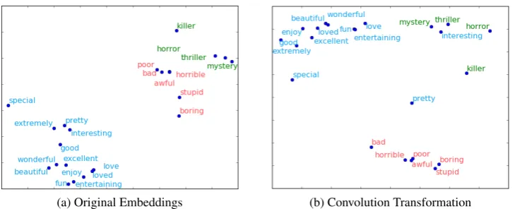
(a) Original Embeddings (b) Convolution Transformation

Figure 1: t-SNE projection of original embeddings and after convolution transformation

What it doesn’t learn

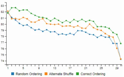
Convolution operation can be explained as a weighted sum across timesteps. This may result in loss of sequential information. To illustrate our hypothesis, we conduct an experiment on the Rot-ten Tomatoes dataset (Pang and Lee,2005). In this experiment we train a CNN with convolution be-ing applied on words with the fixed window size varying from one to maximum sentence length. We repeat this experiment with randomly shuf-fling all the words in an input sentence (Random ordering), and with shuffling every two consecu-tive words as shown in this example “read book forget movie” to “book read movie forget” (Alter-nate shuffle). The results of this experiment are illustrated in Figure 21. Our observations in this experiment are the following:

• CNNs fail to fully incorporate sequential in-formation as performance on random order-ing and correct orderorder-ing are marginally near each other. As evident in the figure, the per-formance with correct ordering on window size 7 is comparable to performance with ran-dom ordering on window size 1.

• As window size increases, the difference be-tween correct and incorrect orderings dimin-ishes and finally converges when window size is complete sentence length. This indi-cates that the ability to capture sequential in-formation by CNNs, decline with increasing window size.

Furthermore, we also note that while performance on random ordering is marginally less than correct

1_{Experiment on more datasets could be found in the}

Ap-pendixB

ordering, it is still higher than other context blind algorithms like bag-of-words as shown in Table

1. This implies that while not fully exploiting se-quential information, convolution filters still learn something valuable which we explore in next sec-tion.

What it learns

To understand what convolution filters do, we train a CNN with single window size on the SST2 dataset (Socher et al.,2013) for sentiment classifi-cation. As the convolution acts over a single word, it has no ability to capture sequential information. Hence, irrespective of input sentence word order, words will always have same respective convo-lution output. Essentially, convoconvo-lution layer here acts like an embedding transformation, where in-put embedding space is transformed into another space. To understand this new space we project the respective embeddings using t-SNE (Maaten and Hinton, 2008) and illustrate them in Figure

1. Here we make a distinction between the se-mantic knowledge of a word and the task spe-cific knowledge of a word. As this experiment is done on dataset SST2, we refer to task specific knowledge as the sentiment knowledge of a word. Word embeddings2 are generally trained on huge domain generic data because of which they cap-ture the general semantic information of the word. Figure1a shows these word embeddings as they are in the original space. As we can see, seman-tically similar words cluster together. Figure 1b shows words after their convolutional transforma-tion. Blue coloured words represent words with positive sentiment. Red with negative sentiment

Figure 2: Accuracy (y-axis) percentage on Rotten Tomatoes dataset with varying window size.

and green words are those which are semantically close to negative sentiment words. However, in the context of movie reviews, their sentiment value is close to positive sentiment words. From this ex-periment we observe:

• The transformation of the green words be-tween original and convoluted outputs, shows that the convolution layer is able to tune their input embeddings such that they are more closer to the positive sentiment cluster than to their original semantic cluster. For exam-ple, a word like “killer” in the original em-bedding space is very close to negative sen-timent words like, “bad” and “awful”, espe-cially if the word embeddings were produced on huge fact based datasets like Wikipedia or news datasets. However in the SST2 dataset, “killer” is often used to describe a movie very positively. Hence sequential learning on such transformed embeddings will be more effec-tive than the original semantic embeddings.

• Some words like “pretty” might be semanti-cally closer to the positive sentiment words. However in the dataset, we find common oc-currences of phrases like “pretty good” or “pretty bad”. The layer has hence trans-formed its position nearly equidistant to both the negative and positive clusters. In other words, convolution layer is able to robustly create a transformation which can handle any task specific noise.

The above observations show the effectiveness of the convolution operation. This is because a single convolution filter output value captures a weighted summation over all the features of the original word embedding. This enables the net-work to learn more task appropriate features as

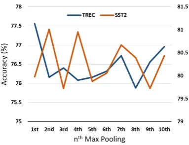
Figure 3: Accuracy (y-axis) percentage on TREC and SST2 datasets with varyingnfor thenthMax pooling.

many as the number of filters.

With the above points in mind, we observe that convolution operation does not fully exploit se-quential information, especially on larger window sizes. However we do see their effectiveness in conforming the input embeddings to a represen-tation specifically meaningful to the task. Hence, for sequential learning instead of relying on con-volution, we use recurrent architectures in our pro-posed SCARN model.

3.2 Max pooling operation: More doesn’t mean better

Max pooling operation in images identify the discriminative features from convolution outputs. However this does not relate the same way of selecting most relevant features from convoluted features in texts. To illustrate this, we perform an experiment using a CNN architecture based on architecture by Kim(2014) popularly used in text classification. We define nth Max pooling as choosingnth highest value of all filters as op-posed to first (n=1). By analyzing the performance distinctions on varying values of n, we make an attempt to assess whether maximum necessarily means task meaningful. The results are illustrated in Figure33. The results show that whennis in-creased the performance varies arbitrarily on all datasets. This shows that there is no apparent co-relation between magnitude of the values to im-portance for the task. Hence, this relationship does not stand strong for text based inputs.

3_{Experiment on more datasets could be found in the}

4 Model

4.1 Overview

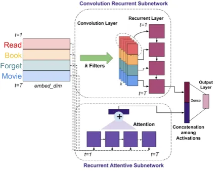
The proposed SCARN model architecture is shown in the Figure4. LetV be the vocabulary size considered and X ∈RV×drepresent

embed-ding matrix whereXiis addimensional word vec-tor. Vocabulary words contained in the pretrained embeddings are initialized to their respective em-bedding vectors and words that are not present are assigned 0’s. For each input text, a maximum lengthN is considered. Zero padding is applied if the length of input text is less thanN. Hence, each sentence or paragraph is converted to I ∈ _RN×d dimensional vector which is the input to SCARN model.

The model consists of two subnetworks: Con-volution Recurrent subnetwork and Recurrent At-tentive subnetwork. In the first subnetwork, con-volution with single window size is applied on the input I. Convolution filters learn the higher level representations from the input text. The out-put from convolution is trained sequentially us-ing LSTM network. In the second subnetwork, the input I is trained using LSTM. To better fo-cus on most relevant words, attention mechanism is applied to the outputs of LSTM from every time step. Attention creates an alternate context vec-tor for the inputI by choosing the most suitable words necessary for classification. The outputs from the first subnetwork and second subnetwork are concatenated and connected to the output layer through a dense connection.

4.2 Convolution Recurrent subnetwork

Let I be represented as sequence of words I =

w1w2w3...wN wherewirepresent theith word in the input. A total ofK convolution filters are ap-plied on each wordwiof input. LetL∈RK×dbe

the weight matrices of all filters. For each filterl

∈_R1×d_{when applied onwi, outputs a new feature}

Cil. Therefore, a new feature vectorCiis obtained for each wordwiafter convolving withKfilters.

Ci=Ci1Ci2Ci3...CiK (1)

Similarly, the above procedure is repeated for all the words in the input to produce a feature vector

C∈_RN×d×K_.

C =f(I~L) (2)

where~represents convolution operation andfis the non-linear activation (ReLU). Applying

con-Figure 4: SCARN Architecture

Figure 5: concat-SCARN architecture

volution to individual words preserve the sequen-tial information. Convolution learns the higher level representations for the input words. Each word will be transformed to a new representation pertinent to the task. The new feature representa-tions are trained sequentially using LSTM.

4.3 Recurrent Attentive subnetwork

In this subnetwork, the input word embeddings are trained using LSTM. All words in the input sentence are not equally important in predicting final output. Although, LSTM learns sequential information, selecting significant information is a key issue for text classification. For this purpose, we employ an attention layer on the top of LSTM outputs. Attention mechanism focuses on specific significant words and tries to construct alternate context vector by aggregating the word represen-tations.

5 Experiments

5.1 Datasets

We tested our model on standard benchmark datasets: Rotten-Tomatoes (RT) (Pang and Lee,

and Subjectivity Objectivity (SO) (Pang and Lee,

2004). The statistics for the datasets are shown in Table3

5.2 Baselines

We compared our model to various text classifica-tion approaches4.

BoW and TF-IDF + LR

Bag-of-words(BoW) and TF-IDF are strong base-lines for text classification. BoW and TF-IDF fea-tures are extracted and softmax is applied on the top for classification.

Average Word Vectors + MLP

This baseline uses the average of word embed-dings as features for the input text which are then trained using Multilayer perceptron (MLP).

Paragraph2Vec + MLP

Each input sentence is converted to a feature vec-tor using Paragraph2vec(Le and Mikolov, 2014) which are then trained using Multilayer perceptron (MLP).

Deep CNN

This baseline is based on deep CNN architecture (Conneau et al.,2016) with approximately match-ing number of parameters as our model.

Char CNN

For our comparison, we employed the Char CNN architecture (Zhou et al.,2015) with less parame-ters compared to the original model, as the datasets used by them were considerably huge than ours.

LSTM and Bi-LSTM

We also offer a comparison with LSTM and Bi-LSTM architectures with a single hidden layer and approximately matching number of parameters as our model.

LSTM + Attention

In this baseline, attention mechanism is applied on the top of LSTM outputs across different time steps.

concat-SCARN

In this model, we concatenate the outputs from convolution layer as in SCARN, with input word embeddings at each time step. The concatenated

4_{For lack of code, results are from our implementations}

outputs are trained using LSTM. Attention is ap-plied on the top of this layer. Figure5shows the architecture of concat-SCARN model.

RCNN

We compared our model to the RCNN model (Lai et al.,2015) which uses max pooling for selecting the most appropriate features of a sentence.

C-LSTM

We compared our model to C-LSTM model (Zhou et al., 2015) which uses convolution over fixed window of words to learn higher level represen-tations.

5.3 Implementation

Input and Training Details

We used google pretrained word vectors for C-LSTM5, as it was used in the original work. For all the other experiments which require embeddings, we use GloVe pretrained word vectors6. The size of a word embedding in this model is 300. For each dataset, a maximum sentence length is con-sidered which is 30 for TREC, SO, RT, Pol, SST-2 datasets, 400 for IMDB and 100 for AR dataset.

We apply a dropout layer (Srivastava et al.,

2014) with a probability of 0.5 on the pretrained embeddings. We also apply dropout with a prob-ability 0.5 on the dense layer that connects to out-put. We use Adam as the optimizer with a batch-size of 16 for small SCARN model and 50 for Large SCARN model. The initial learning rate is set to 0.0003. Training is done for 30 epochs.

Architecture

We employ two different architectures of SCARN model since the datasets vary in size. For datasets TREC, SO, RT, Pol, SST-2 the number of convo-lution filters are 50. Number of LSTM cells con-sidered for these datasets are 32. We call this ar-chitectureSmall SCARN model. For datasets AR and IMDB, number of convolution filters are 100 and number of LSTM cells are 64. We call this architectureLarge SCARN model. The compar-ison of number of parameters for each model is shown in Table2. ReLU is used as the activation function in convolution layers. In the output layer, softmax is used for multi-class classification and sigmoid for binary.

5

https://code.google.com/archive/p/word2vec/

Model IMDB TREC SO RT Pol AR SST-2

Linear BoW + LR 86.452 73.600 82.800 64.320 76.500 47.000 80.500 TFIDF + LR 78.740 72.000 84.000 63.237 77.250 49.200 80.340

Word Vector Avg Word Vectors + MLP 85.44 86.999 90 75.691 68.25 47.015 81.219 Paragraph2Vec + MLP 77.472 45 77.2 62.996 77.25 38.925 67.27

CNN Deep CNN 78.44 28.999 85.799 75.4 69.999 40.333 64.305

Char CNN 70.484 74.199 59 50 50.249 34.37 60.516

RNN LSTM 88.37 76.99 90.899 77.436 74.5 47.85 78.747

Bi-LSTM 88.69 75.8 91.399 76.594 77.499 51.569 79.242

Attention LSTM+Attention 88.35 77 89.7 76.895 77.75 50.568 80.01 concat-SCARN 88.88 78.8 89.8 77.858 75.75 51.569 80.06

RNN-CNN RCNN 86.607 79.6 91.1 78.098 78.25 48.026 80.395

C-LSTM 87.676 90.4 91.3 76.474 67 52.784 78.308

Our model SCARN 89.788 90.799 92.4 79.641 78.75 53.350 82.262

Table 1: Accuracy scores in percentage of all models on every dataset

Figure 6: Attention weights for some of the sentences from the SST2 dataset

Model No. of parameters

Small SCARN 68,425

Large SCARN 166,639

RCNN 180,601

C-LSTM 676,651

Table 2: Number of parameters for each model

6 Results and Discussion

Results of the experiments are tabulated in Table

1. We observe that, the proposed SCARN model outperforms linear and word vector based models, because of their inability to incorporate sequential information. We also compare our model to recur-rent models like LSTM, Bidirectional-LSTM and find that SCARN outperforms them as these re-current architectures even though learn sequential information, lack SCARN’s learning of task spe-cific representations through convolution. Mean-while, SCARN outperforms deep CNN and char CNN models, for their lack of learning

sequen-tial information the same way recurrent architec-tures can. When SCARN is compared to other re-current convolutional architectures RCNN and C-LSTM, SCARN achieves significantly much bet-ter performance with lesser paramebet-ters as shown in Table2. RCNN uses max pooling to capture the most important feature. However our discussions in Section3.2show max pooling’s choice of max-imum may not necessitate importance. C-LSTM used fixed window convolution across words. But as seen in Section 3.1 fixed window convolution do not capture sequential information adequately. In SCARN model, we apply convolution across single word to learn task specific information, on which LSTM architecture is trained to capture contextual information.

Dataset Dataset size Train Dev Test Max Vocab size Classes

IMDB 50000 20000 5000 25000 30000 2

TREC 5952 4906 546 500 5000 6

SO 10000 8100 900 1000 30000 2

RT 10662 8100 900 1662 30000 2

Pol 2000 1280 320 400 30000 2

AR 121565 80000 20000 21565 30000 5

SST-2 9613 6920 872 1821 10000 2

Table 3: Summary Statistics of all datasets

(a) Mean

(b) Standard Deviation

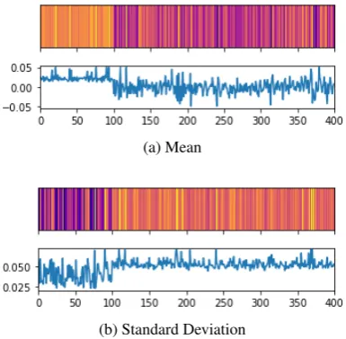
Figure 7: Statistics of each feature in concatenation layer outputs on the IMDB dataset’s training set.

average and standard deviation of outputs at the concatenation layer of concat-SCARN on IMDB dataset’s training set. As evident from the fig-ure, we can make a stark distinction between the two concatenated sections as shown in the archi-tecture of concat-SCARN in Figure 5. Because of the irregular distributions, the learning may be-come biased towards one of the segments. Fur-thermore, attempts to address this issue by using batch normalization layers may not be a good idea, as normalizing word embedding inputs may spoil the semantic concepts underlying them. Hence, in our SCARN model, subnetworks are trained dif-ferently, and final activations are concatenated as illustrated in SCARN’s architecture in Figure 4. As long as both subnetworks’ outputs come from similar activation function, they will have similar distributions as well and hence they won’t suffer from the same problem as concat-SCARN.

Effectiveness of attention has also been illus-trated in Figure 6, where attention weights have been shown in a heat map, with darker colors

cor-responding to a higher weightage. We observe that SCARN is able to effectively utilize attention weights to focus on most contributing input words.

7 Conclusion

In this paper we present a critical study and view-point of CNNs, which even though are popularly used in text classification, details of it are of-ten overlooked. We find that convolutional fil-ters learn particularly in the context of sequen-tial information. But at the same time, they are good at learning higher level task-relevant fea-tures. On the other hand, we find max pooling to be very arbitrary in selection of crucial fea-tures and hence contributing minimal to the over-all task. We also find that the problems with in-put concatenation, as it imbalances the represen-tations because of difference in nature of distribu-tions. Based on our study we proposed SCARN, for effectively utilizing convolution and recurrent features for text classification. Our model beats other popular ways of combining recurrent and convolutional architectures with quite less number of parameters on various benchmark datasets. Our model also outperforms CNN and RNN architec-tures with equally deep or same number of param-eters.

References

Dzmitry Bahdanau, Kyunghyun Cho, and Yoshua Ben-gio. 2014. Neural machine translation by jointly learning to align and translate. arXiv preprint arXiv:1409.0473.

Alexis Conneau, Holger Schwenk, Lo¨ıc Barrault, and Yann Lecun. 2016. Very deep convolutional networks for text classification. arXiv preprint arXiv:1606.01781.

bidirectional transformers for language understand-ing. arXiv preprint arXiv:1810.04805.

Ruining He and Julian McAuley. 2016. Ups and downs: Modeling the visual evolution of fashion trends with one-class collaborative filtering. In proceedings of the 25th international conference on world wide web, pages 507–517. International World Wide Web Conferences Steering Committee.

Sepp Hochreiter and J¨urgen Schmidhuber. 1997. Long short-term memory. Neural computation, 9(8):1735–1780.

Yoon Kim. 2014. Convolutional neural net-works for sentence classification. arXiv preprint arXiv:1408.5882.

Siwei Lai, Liheng Xu, Kang Liu, and Jun Zhao. 2015. Recurrent convolutional neural networks for text classification. InTwenty-ninth AAAI conference on artificial intelligence.

Quoc Le and Tomas Mikolov. 2014. Distributed repre-sentations of sentences and documents. In Interna-tional conference on machine learning, pages 1188– 1196.

Ji Young Lee and Franck Dernoncourt. 2016. Se-quential short-text classification with recurrent and convolutional neural networks. arXiv preprint arXiv:1603.03827.

Xin Li and Dan Roth. 2002. Learning question classi-fiers. InProceedings of the 19th International Con-ference on Computational Linguistics - Volume 1, COLING ’02, pages 1–7, Stroudsburg, PA, USA. Association for Computational Linguistics.

Zhouhan Lin, Minwei Feng, Cicero Nogueira dos San-tos, Mo Yu, Bing Xiang, Bowen Zhou, and Yoshua Bengio. 2017. A structured self-attentive sentence embedding. arXiv preprint arXiv:1703.03130.

Minh-Thang Luong, Hieu Pham, and Christopher D Manning. 2015. Effective approaches to attention-based neural machine translation. arXiv preprint arXiv:1508.04025.

Andrew L. Maas, Raymond E. Daly, Peter T. Pham, Dan Huang, Andrew Y. Ng, and Christopher Potts. 2011. Learning word vectors for sentiment analy-sis. InProceedings of the 49th Annual Meeting of the Association for Computational Linguistics: Hu-man Language Technologies, pages 142–150, Port-land, Oregon, USA. Association for Computational Linguistics.

Laurens van der Maaten and Geoffrey Hinton. 2008. Visualizing data using t-sne. Journal of machine learning research, 9(Nov):2579–2605.

Avinash Madasu and Vijjini Anvesh Rao. 2019a. Effectiveness of self normalizing neural net-works for text classification. arXiv preprint arXiv:1905.01338.

Avinash Madasu and Vijjini Anvesh Rao. 2019b. Gated convolutional neural networks for domain adaptation. InInternational Conference on Applica-tions of Natural Language to Information Systems, pages 118–130. Springer.

Bo Pang and Lillian Lee. 2004. A sentimental educa-tion: Sentiment analysis using subjectivity. In Pro-ceedings of ACL, pages 271–278.

Bo Pang and Lillian Lee. 2005. Seeing stars: Exploit-ing class relationships for sentiment categorization with respect to rating scales. InProceedings of ACL, pages 115–124.

Cicero dos Santos, Ming Tan, Bing Xiang, and Bowen Zhou. 2016. Attentive pooling networks. arXiv preprint arXiv:1602.03609.

Richard Socher, Alex Perelygin, Jean Wu, Jason Chuang, Christopher D Manning, Andrew Ng, and Christopher Potts. 2013. Recursive deep models for semantic compositionality over a sentiment tree-bank. In Proceedings of the 2013 conference on empirical methods in natural language processing, pages 1631–1642.

Nitish Srivastava, Geoffrey Hinton, Alex Krizhevsky, Ilya Sutskever, and Ruslan Salakhutdinov. 2014. Dropout: a simple way to prevent neural networks from overfitting. The Journal of Machine Learning Research, 15(1):1929–1958.

Christian Szegedy, Vincent Vanhoucke, Sergey Ioffe, Jon Shlens, and Zbigniew Wojna. 2016. Rethink-ing the inception architecture for computer vision. InProceedings of the IEEE conference on computer vision and pattern recognition, pages 2818–2826.

Sida Wang and Christopher D Manning. 2012. Base-lines and bigrams: Simple, good sentiment and topic classification. In Proceedings of the 50th Annual Meeting of the Association for Computational Lin-guistics: Short Papers-Volume 2, pages 90–94. As-sociation for Computational Linguistics.

Zichao Yang, Diyi Yang, Chris Dyer, Xiaodong He, Alex Smola, and Eduard Hovy. 2016. Hierarchi-cal attention networks for document classification. InProceedings of the 2016 Conference of the North American Chapter of the Association for Computa-tional Linguistics: Human Language Technologies, pages 1480–1489.

Xiang Zhang, Junbo Zhao, and Yann LeCun. 2015. Character-level convolutional networks for text clas-sification. In Advances in neural information pro-cessing systems, pages 649–657.

(a) RT (b) IMDB (c) SO

Figure 8:nth_{Max pooling experiments on RT, IMDB and SO Datasets}

Figure 9: Percentage distribution of max pooling out-puts for misclassified samples from SST2 dataset

A Max Pooling: missclassified examples

For this experiment, after convolution over sin-gle word, we perform max pooling across filter outputs and attempt to discern the max pooling outputs. We identify which input words’ convo-lution outputs were chosen by the max pooling operation. These distributions illustrated in Fig-ure 9are presented on some misclassified exam-ples from the SST2 dataset. We see that often words that should have been contributing most to the overall sentiment value, have very less or min-imal share. For example in the sentence, “it is also stupider”, we see “is” having the near majority share, even though it tells nothing about the sen-timent of the sentence. At the same time in “rainy days and movies about the disintegration of fami-lies always get me down”, “disintegration” has al-most no share despite being an important word for evaluating sentiment.

B Experiments on more datasets

Figure8 shows the nth _{Max pooling experiment} explained in Section3.2on other datasets, namely RT, IMDB and SO. We still find that there is no

Figure 10: Accuracy (y-axis) percentage on SO dataset with varying window size.

Figure 11: Accuracy (y-axis) percentage on SST2 dataset with varying window size.