Proceedings of the 2019 Conference on Empirical Methods in Natural Language Processing
4282
FlowSeq: Non-Autoregressive Conditional
Sequence Generation with Generative Flow
Xuezhe Ma⇤,1 Chunting Zhou⇤,1 Xian Li2 Graham Neubig1 Eduard Hovy1 1Language Technologies Institute, Carnegie Mellon University
2Facebook AI
{xuezhem, chuntinz, gneubig, ehovy}@cs.cmu.edu [email protected]
Abstract
Most sequence-to-sequence (seq2seq) models are autoregressive; they generate each token by conditioning on previously generated to-kens. In contrast, non-autoregressive seq2seq models generate all tokens in one pass, which leads to increased efficiency through parallel processing on hardware such as GPUs. How-ever, directly modeling the joint distribution of all tokens simultaneously is challenging, and even with increasingly complex model struc-tures accuracy lags significantly behind au-toregressive models. In this paper, we propose a simple, efficient, and effective model for non-autoregressive sequence generation using latent variable models. Specifically, we turn to generative flow, an elegant technique to model complex distributions using neural net-works, and design several layers of flow tai-lored for modeling the conditional density of sequential latent variables. We evaluate this model on three neural machine translation (NMT) benchmark datasets, achieving com-parable performance with state-of-the-art non-autoregressive NMT models and almost con-stant decoding time w.r.t the sequence length.1
1 Introduction
Neural sequence-to-sequence (seq2seq) models (Bahdanau et al.,2015;Rush et al.,2015;Vinyals et al., 2015; Vaswani et al., 2017) generate an output sequence y = {y1, . . . , yT} given an in-put sequence x = {x1, . . . , xT0} using condi-tional probabilities P✓(y|x) predicted by neural
networks (parameterized by✓).
Most seq2seq models areautoregressive, mean-ing that they factorize the joint probability of the output sequence given the input sequenceP✓(y|x)
into the product of probabilities over the next
to-⇤Equal contribution, in alphabetical order.
1https://github.com/XuezheMax/flowseq
(a)
(c)
(b)
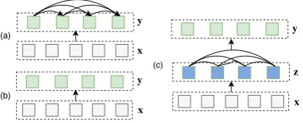
Figure 1: (a) Autoregressive (b) non-autoregressive and (c) our proposed sequence generation models. xis the
source,yis the target, andzare latent variables.
ken in the sequence given the input sequence and previously generated tokens:
P✓(y|x) = T
Y
t=1
P✓(yt|y<t,x). (1)
Each factor,P✓(yt|y<t,x), can be implemented by function approximators such as RNNs ( Bah-danau et al., 2015) and Transformers (Vaswani et al., 2017). This factorization takes the com-plicated problem of joint estimation over an ex-ponentially large output space of outputs y, and turns it into a sequence of tractable multi-class classification problemspredictingytgiven the pre-vious words, allowing for simple maximum log-likelihood training. However, this assumption of left-to-right factorization may be sub-optimal from a modeling perspective (Gu et al., 2019; Stern et al.,2019), and generation of outputs must be done through a linear left-to-right pass through the output tokens using beam search, which is not easily parallelizable on hardware such as GPUs.
Recently, there has been work on non-autoregressive sequence generation for neural ma-chine translation (NMT; Gu et al. (2018); Lee et al.(2018);Ghazvininejad et al.(2019)) and lan-guage modeling (Ziegler and Rush,2019). Non-autoregressive models attempt to model the joint distribution P✓(y|x) directly, decoupling the
[image:1.595.309.526.223.311.2]A na¨ıve solution is to assume that each token of the target sequence is independent given the input:
P✓(y|x) = T
Y
t=1
P✓(yt|x). (2)
Unfortunately, the performance of this simple model falls far behind autoregressive models, as seq2seq tasks usually do have strong conditional dependencies between output variables (Gu et al., 2018). This problem can be mitigated by introduc-ing a latent variablez to model these conditional dependencies:
P✓(y|x) =
Z
z
P✓(y|z,x)p✓(z|x)dz, (3)
where p✓(z|x) is the prior distribution over
la-tent z and P✓(y|z,x) is the “generative”
distri-bution (a.k.a decoder). Non-autoregressive gen-eration can be achieved by the following indepen-dence assumption in the decoding process:
P✓(y|z,x) = T
Y
t=1
P✓(yt|z,x). (4)
Gu et al. (2018) proposed az representing fertil-ity scores specifying the number of output words each input word generates, significantly improv-ing the performance over Eq. (2). But the per-formance still falls behind state-of-the-art autore-gressive models due to the limited expressiveness of fertility to model the interdependence between words iny.
In this paper, we propose a simple, effective, and efficient model, FlowSeq, which models ex-pressive prior distribution p✓(z|x) using a
pow-erful mathematical framework called generative flow (Rezende and Mohamed,2015). This frame-work can elegantly model complex distributions, and has obtained remarkable success in model-ing continuous data such as images and speech through efficient density estimation and sampling (Kingma and Dhariwal,2018;Prenger et al.,2019; Ma and Hovy, 2019). Based on this, we posit that generative flow also has potential to introduce more meaningful latent variables z in the non-autoregressive generation in Eq. (3).
FlowSeq is a flow-based sequence-to-sequence
model, which is (to our knowledge) the first non-autoregressive seq2seq model utilizing gen-erative flows. It allows for efficient parallel decoding while modeling the joint distribution of the output sequence. Experimentally, on
three benchmark datasets for machine transla-tion – WMT2014, WMT2016 and IWSLT-2014, FlowSeq achieves comparable performance with state-of-the-art non-autoregressive models, and al-most constant decoding time w.r.t. the sequence length compared to a typical left-to-right Trans-former model, which is super-linear.
2 Background
As noted above, incorporating expressive latent variables z is essential to decouple the depen-dencies between tokens in the target sequence in non-autoregressive models. However, in order to model all of the complexities of sequence gener-ation to the point that we can read off all of the words in the output in an independent fashion (as in Eq. (4)), the prior distributionp✓(z|x)will
nec-essarily be quite complex. In this section, we de-scribe generative flows (Rezende and Mohamed, 2015), an effective method for arbitrary model-ing of complicated distributions, before describmodel-ing how we apply them to sequence-to-sequence gen-eration in§3.
2.1 Flow-based Generative Models
Put simply, flow-based generative models work by transforming a simple distribution (e.g. a simple Gaussian) into a complex one (e.g. the complex prior distribution over z that we want to model) through a chain of invertible transformations.
Formally, a set of latent variables 2 ⌥are
introduced with a simple prior distributionp⌥( ).
We then define a bijection function f : Z ! ⌥
(withg=f 1), whereby we can define a genera-tive process over variablesz:
⇠ p⌥( )
z = g✓( ). (5)
An important insight behind flow-based models is that given this bijection function, the change of variable formula defines the model distribution on z2Z by:
p✓(z) =p⌥(f✓(z)) det(
@f✓(z)
@z ) . (6) Here @f✓(z)
@z is the Jacobian matrix off✓atz.
g✓ and the Jacobian determinants are tractable to
compute. A stacked sequence of such invert-ible transformations is also called a (normalizing)
flow(Rezende and Mohamed,2015):
z !f1
g1
H1 !f2
g2
H2 !f3
g3 · · ·
fK
!
gK ,
wheref =f1 f2 · · · fKis a flow ofK trans-formations (omitting✓s for brevity).
2.2 Variational Inference and Training
In the context of maximal likelihood estimation (MLE), we wish to minimize the negative log-likelihood of the parameters:
min
✓2⇥
1
N
N
X
i=1
logP✓(yi|xi), (7)
where D = {(xi,yi)}Ni=1 is the set of
train-ing data. However, the likelihood P✓(y|x)
af-ter marginalizing out latent variables z (LHS in Eq. (3)) is intractable to compute or differentiate directly. Variational inference (Wainwright et al., 2008) provides a solution by introducing a para-metric inference model q (z|y,x) (a.k.a
poste-rior) which is then used to approximate this inte-gral by sampling individual examples ofz. These models then optimize the evidence lower bound
(ELBO), which considers both the “reconstruction error”logP✓(y|z,x)and KL-divergence between
the posterior and the prior:
logP✓(y|x) Eq (z|y,x)[logP✓(y|z,x)]
KL(q (z|y,x)||p✓(z|x)). (8)
Both inference model and decoder✓parameters
are optimized according to this objective.
3 FlowSeq
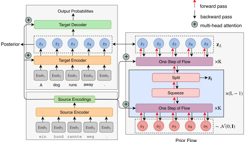
We first overview FlowSeq’s architecture (shown in Figure 2) and training process here before detailing each component in following sections. Similarly to classic seq2seq models, at both traing and test time FlowSeq first reads the whole in-put sequence x and calculates a vector for each word in the sequence, the source encoding.
At training time, FlowSeq’s parameters are learned using a variational training paradigm overviewed in§2.2. First, we draw samples of la-tent codeszfrom the current posteriorq (z|y,x).
Next, we feed z together with source encod-ings into the decoder network and the prior flow
to compute the probabilities of P✓(y|z,x) and
p✓(z|x)for optimizing the ELBO (Eq. (8)).
At test time, generation is performed by first sampling a latent codezfrom the prior flow by ex-ecuting the generative process defined in Eq. (5). In this step, the source encodings produced from the encoder are used as conditional inputs. Then the decoder receives both the sampled latent code z and the source encoder outputs to generate the target sequenceyfromP✓(y|z,x).
3.1 Source Encoder
The source encoder encodes the source sequences into hidden representations, which are used in computing attention when generating latent vari-ables in the posterior network and prior network as well as the cross-attention with decoder. Any standard neural sequence model can be used as its encoder, including RNNs (Bahdanau et al.,2015) or Transformers (Vaswani et al.,2017).
3.2 Posterior
Generation of Latent Variables. The latent variableszare represented as a sequence of con-tinuous random vectorsz={z1, . . . ,zT}with the same length as the target sequence y. Eachztis a dz-dimensional vector, where dz is the dimen-sion of the latent space. The posterior distribution
q (z|y,x)models eachztas a diagonal Gaussian with learned mean and variance:
q (z|y,x) =
T
Y
t=1
N(zt|µt(x,y), t2(x,y)) (9)
whereµt(·)and t(·)are neural networks such as RNNs or Transformers.
Zero initialization. While we perform standard random initialization for most layers of the net-work, we initialize the last linear transforms that generate theµandlog 2 values with zeros. This
ensures that the posterior distribution as a simple normal distribution, which we found helps train very deep generative flows more stably.
A dog runs away . Target Encoder Target Decoder Output Probabilities
One Step of Flow Squeeze
Split One Step of Flow
ein hund rannte weg . Source Encoder Source Encodings
+
+
forward pass
backward pass
multi-head attention
Prior Flow +
+
[image:4.595.90.507.64.305.2]+ Posterior
Figure 2: Neural architecture of FlowSeq, including the encoder, the decoder and the posterior networks, together with the multi-scale architecture of the prior flow. The architecture of each flow step is in Figure3.
“correct” token at each steptwithztas input. In this case, FlowSeq reduces to the baseline model in Eq. (2). To escape this undesired local opti-mum, we apply token-level dropout to randomly drop an entire token when calculating the poste-rior, to ensure the model also has to learn how to use contextual information. This technique is sim-ilar to the “masked language model” in previous studies (Melamud et al.,2016;Devlin et al.,2018; Ma et al.,2018).
3.3 Decoder
As the decoder, we take the latent sequence z as input, run it through several layers of a neural se-quence model such as a Transformer, then directly predict the output tokens inyindividually and in-dependently. Notably, unlike standard seq2seq de-coders, we do not perform causal masking to pre-vent attending to future tokens, making the model fully non-autoregressive.
3.4 Flow Architecture for Prior
The flow architecture is based on Glow (Kingma and Dhariwal,2018). It consists of a series of steps of flow, combined in a multi-scale architecture (see Figure 2.) Each step of flow consists three types of elementary flows – actnorm, invertible multi-head linear, and coupling. Note that all three functions are invertible and conducive to calcula-tion of log determinants (details in AppendixA).
Actnorm. The activation normalization layer (actnorm; Kingma and Dhariwal (2018)) is an alternative for batch normalization (Ioffe and Szegedy,2015), that has mainly been used in the context of image data to alleviate problems in model training. Actnorm performs an affine trans-formation of the activations using a scale and bias parameter per feature for sequences:
z0t=s zt+b. (10)
Bothzandz0 are tensors of shape[T ⇥dz]with time dimensiont and feature dimensiondz. The parameters are initialized such that over each fea-ture z0
t has zero mean and unit variance given an initial mini-batch of data.
Invertible Multi-head Linear Layers. To in-corporate general permutations of variables along the feature dimension to ensure that each dimen-sion can affect every other ones after a sufficient number of steps of flow, Kingma and Dhariwal (2018) proposed a trainable invertible1⇥1
convo-lution layer for 2D images. It is straightforward to apply similar transformations to sequential data:
z0t=ztW, (11)
whereWis the weight matrix of shape[dz⇥dz]. The log-determinant of this transformation is:
log det
✓@linear(z;W)
@z
◆
=T·log|det(W)|
Encoder Inter-Attention
source encodings
ActNorm Linear Layer Affine Coupling Layer
(a) One step of flow. (b) Coupling layer splits. (c) NN function on the split of the coupling layer.
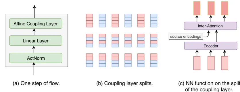
Figure 3: (a) The architecture of one step of our flow. (b) The visualization of three split pattern for coupling layers, where the red color denotesza and the blue color denoteszvb. (c) The attention-based architecture of the
NN function in coupling layers.
Unfortunately, dz in Seq2Seq generation is commonly large, e.g. 512, significantly slowing
down the model for computingdet(W). To apply
this to sequence generation, we propose a multi-head invertible linear layer, which first splits each
dz-dimensional feature vector into h heads with dimension dh = dz/h. Then the linear trans-formation in (11) is applied to each head, with
dh ⇥ dh weight matrix W, significantly reduc-ing the dimension. For splittreduc-ing of heads, one step of flow contains one linear layer with either row-major or column-row-major splitting format, and these steps with different linear layers are composed in an alternating pattern.
Affine Coupling Layers. To model interdepen-dence across time steps, we use affine coupling layers (Dinh et al.,2016):
za,zb = split(z) z0a = za
z0b = s(za,x) zb+ b(za,x) z0 = concat(z0a,z0b),
where s(za,x) and b(za,x) are outputs of two neural networks withzaandxas input. These are shown in Figure3(c). In experiments, we imple-ments(·) andb(·) with one Transformer decoder
layer (Vaswani et al., 2017): multi-head self-attention over za, followed by multi-head inter-attention overx, followed by a position-wise feed-forward network. The inputzais fed into this layer in one pass, without causal masking.
As in Dinh et al. (2016), the split() function
splitszthe input tensor into two halves, while the
concat operation performs the corresponding
re-verse concatenation operation. In our architecture, three types of split functions are used, based on
the split dimension and pattern. Figure 3 (b) il-lustrates the three splitting types. The first type of split groupsz along the time dimension on alter-nate indices. In this case, FlowSeq mainly models the interactions between time-steps. The second and third types of splits perform on the feature di-mension, with continuous and alternate patterns, respectively. For each type of split, we alternateza andzb to increase the flexibility of the split func-tion. Different types of affine coupling layers al-ternate in the flow, similar to the linear layers.
Multi-scale Architecture. We followDinh et al. (2016) in implementing a multi-scale architecture using the squeezing operation on the feature di-mension, which has been demonstrated helpful for training deep flows. Formally, each scale is a com-bination of several steps of the flow (see Figure3 (a)). After each scale, the model drops half of the dimensions with the third type of split in Figure3 (b) to reduce computational and memory cost, out-putting the tensor with shape [T ⇥ d2]. Then the
squeezing operation transforms theT ⇥ d2 tensor
into an T
2⇥done as the input of the next scale. We pad each sentence withEOStokens to ensureTis
divisible by 2. The right component of Figure2
illustrates the multi-scale architecture.
3.5 Predicting Target Sequence Length
[image:5.595.83.501.61.222.2]and target sequences using a classifier with a range of[ 20,20]. Numbers in this range are predicted
by max-pooling the source encodings into a single vector,2 running this through a linear layer, and taking a softmax. This classifier is learned jointly with the rest of the model.
3.6 Decoding Process
At inference time, the model needs to identify the sequence with the highest conditional probability by marginalizing over all possible latent variables (see Eq. (3)), which is intractable in practice. We propose three approximating decoding algorithms to reduce the search space.
Argmax Decoding. FollowingGu et al.(2018), one simple and effective method is to select the best sequence by choosing the highest-probability latent sequencez:
z⇤ = argmax
z2Z
p✓(z|x)
y⇤ = argmax
y P✓(y|z
⇤,x)
where identifyingy⇤only requires independently maximizing the local probability for each output position (see Eq.4).
Noisy Parallel Decoding (NPD). A more accu-rate approximation of decoding, proposed in Gu et al. (2018), is to draw samples from the latent space and compute the best output for each la-tent sequence. Then, a pre-trained autoregres-sive model is adopted to rank these sequences. In FlowSeq, different candidates can be generated by sampling different target lengths or different sam-ples from the prior, and both of the strategies can be batched via masks during decoding. In our experiments, we first select the top l length
can-didates from the length predictor in §3.5. Then, for each length candidate we use r random sam-ples from the prior network to generate output se-quences, yielding a total ofl⇥rcandidates.
Importance Weighted Decoding (IWD) The third approximating method is based on thelower bound of importance weighted estimation(Burda et al.,2015). Similarly to NPD, IWD first draws samples from the latent space and computes the best output for each latent sequence. Then, IWD
2We experimented with other methods such as
mean-pooling or taking the last hidden state and found no major difference in our experiments
ranks these candidate sequences with K impor-tance samples:
zi ⇠ p✓(z|x),8i= 1, . . . , N
ˆ
yi = argmax
y P✓(y|zi,x)
zi(k) ⇠ q (z|yiˆ ,x),8k= 1, . . . , K P(ˆyi|x) ⇡ K1
K
P
k=1
P✓(ˆyi|z(ik),x)p✓(z(ik)|x) q (z(ik)|yˆi,x)
IWD does not rely on a separate pre-trained model, though it significantly slows down the de-coding speed. The detailed comparison of these three decoding methods is provided in§4.2.
3.7 Discussion
Different from the architecture proposed inZiegler and Rush (2019), the architecture of FlowSeq is not using any autoregressive flow (Kingma et al., 2016; Papamakarios et al., 2017), yield-ing a truly non-autoregressive model with efficient generation. Note that the FlowSeq remains non-autoregressive even if we use an RNN in the ar-chitecture because RNN is only used to encode a complete sequence of codes and all the input to-kens can be fed into the RNN in parallel. This makes it possible to use highly-optimized imple-mentations of RNNs such as those provided by cuDNN.3 Thus while RNNs do experience some drop in speed, it is less extreme than that experi-enced when using autoregressive models.
4 Experiments
4.1 Experimental Setups
Translation Datasets We evaluate FlowSeq on three machine translation benchmark datasets: WMT2014 DE-EN (around 4.5M sentence pairs), WMT2016 RO-EN (around 610K sentence pairs) and a smaller dataset IWSLT2014 DE-EN (around 150K sentence pairs). We use scripts from fairseq (Ott et al., 2019) to preprocess WMT2014 and IWSLT2014, where the preprocessing steps fol-low Vaswani et al. (2017) for WMT2014. We use the data provided in Lee et al. (2018) for WMT2016. For both WMT datasets, the source and target languages share the same set of BPE embeddings while for IWSLT2014 we use sepa-rate embeddings. During training, we filter out sentences longer than80for WMT dataset and60
for IWSLT, respectively.
3
WMT2014 WMT2016 IWSLT2014 Models EN-DE DE-EN EN-RO RO-EN DE-EN
Raw Data
CMLM-base 10.88 – 20.24 – –
LV NAR 11.80 – – – –
FlowSeq-base 18.55 23.36 29.26 30.16 24.75 FlowSeq-large 20.85 25.40 29.86 30.69 –
Knowledge Distillation
[image:7.595.71.289.63.233.2]NAT-IR 13.91 16.77 24.45 25.73 21.86 CTC Loss 17.68 19.80 19.93 24.71 – NAT w/ FT 17.69 21.47 27.29 29.06 20.32 NAT-REG 20.65 24.77 – – 23.89 CMLM-small 15.06 19.26 20.12 20.36 – CMLM-base 18.12 22.26 23.65 22.78 – FlowSeq-base 21.45 26.16 29.34 30.44 27.55 FlowSeq-large 23.72 28.39 29.73 30.72 –
Table 1: BLEU scores on three MT benchmark datasets for FlowSeq with argmax decoding and baselines with purely non-autoregressive decoding method. The first and second block are results of models trained w/w.o. knowledge distillation, respectively.
Modules and Hyperparameters We imple-ment the encoder, decoder and posterior net-works with standard (unmasked) Transformer lay-ers (Vaswani et al., 2017). For WMT datasets, the encoder consists of 6 layers, and the decoder and posterior are composed of 4 layers, and 8 attention heads. and for IWSLT, the encoder has 5 layers, and decoder and posterior have 3 layers, and 4 attention heads. The prior flow consists of 3 scales with the number of steps
[48,48,16]from bottom to top. To dissect the
im-pact of model dimension on translation quality and speed, we perform experiments on two versions of FlowSeq withdmodel/dhidden = 256/512(base) and dmodel/dhidden = 512/1024 (large). More model details are provided in AppendixB.
Optimization Parameter optimization is per-formed with the Adam optimizer (Kingma and Ba, 2014) with = (0.9,0.999)and✏= 1e 6. Each
mini-batch consist of 2048sentences. The
learn-ing rate is initialized to5e 4, and exponentially
decays with rate0.999995. The gradient clipping
cutoff is1.0. For all the FlowSeq models, we
ap-ply 0.1 label smoothing and averaged the 5 best
checkpoints to create the final model.
At the beginning of training, the posterior net-work is randomly initialized, producing noisy su-pervision to the prior. To mitigate this issue, we first set the weight of the KL term in ELBO to
zero for 30,000 updates to train the encoder, de-coder and posterior networks. Then theKLweight
linearly increases to one for another 10,000
up-WMT2014 WMT2016 Models EN-DE DE-EN EN-RO RO-EN
Autoregressive Methods
Transformer-base 27.30 – – – Our Implementation 27.16 31.44 32.92 33.09
Raw Data
CMLM-base (refinement 4) 22.06 – 30.89 – CMLM-base (refinement 10) 24.65 – 32.53 – FlowSeq-base (IWDn= 15) 20.20 24.63 30.61 31.50 FlowSeq-base (NPDn= 15) 20.81 25.76 31.38 32.01 FlowSeq-base (NPDn= 30) 21.15 26.04 31.74 32.45 FlowSeq-large (IWDn= 15) 22.94 27.16 31.08 32.03 FlowSeq-large (NPDn= 15) 23.14 27.71 31.97 32.46 FlowSeq-large (NPDn= 30) 23.64 28.29 32.35 32.91
Knowledge Distillation
NAT-IR (refinement 10) 21.61 25.48 29.32 30.19 NAT w/ FT (NPDn= 10) 18.66 22.42 29.02 31.44 NAT-REG (NPDn= 9) 24.61 28.90 – – LV NAR (refinement 4) 24.20 – – – CMLM-small (refinement 10) 25.51 29.47 31.65 32.27 CMLM-base (refinement 10) 26.92 30.86 32.42 33.06 FlowSeq-base (IWDn= 15) 22.49 27.40 30.59 31.58 FlowSeq-base (NPDn= 15) 23.08 28.07 31.35 32.11 FlowSeq-base (NPDn= 30) 23.48 28.40 31.75 32.49 FlowSeq-large (IWDn= 15) 24.70 29.44 31.02 31.97 FlowSeq-large (NPDn= 15) 25.03 30.48 31.89 32.43 FlowSeq-large (NPDn= 30) 25.31 30.68 32.20 32.84
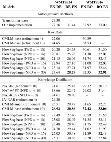
Table 2: BLEU scores on two WMT datasets of models using advanced decoding methods. The first block are Transformer-base (Vaswani et al.,2017). The second and the third block are results of models trained w/w.o. knowledge distillation, respectively. n = l⇥ris the total number of candidates for rescoring.
dates, which we found essential to accelerate train-ing and achieve stable performance.
Knowledge Distillation Previous work on non-autoregressive generation (Gu et al., 2018; Ghazvininejad et al., 2019) has used translations produced by a pre-trained autoregressive NMT model as the training data, noting that this can sig-nificantly improve the performance. We analyze the impact of distillation in§4.2.
4.2 Main Results
We first conduct experiments to compare the per-formance of FlowSeq with strong baseline mod-els, including NAT w/ Fertility (Gu et al.,2018), NAT-IR (Lee et al., 2018), NAT-REG (Wang et al., 2019), LV NAR (Shu et al., 2019), CTC Loss (Libovick`y and Helcl, 2018), and CMLM (Ghazvininejad et al.,2019).
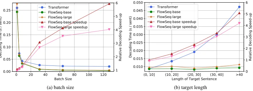
[image:7.595.306.525.63.340.2] [image:7.595.307.525.65.344.2](a) batch size (b) target length
Figure 4: The decoding speed of Transformer (batched, beam size 5) and FlowSeq on WMT14 EN-DE test set (a) w.r.t different batch sizes (b) bucketed by different target sentence lengths (batch size 32).
knowledge distillation. Without using knowledge distillation, FlowSeq base model achieves signif-icant improvement (more than 9 BLEU points)
over CMLM-base and LV NAR. It demonstrates the effectiveness of FlowSeq on modeling the complex interdependence in target languages.
Towards the effect of knowledge distillation, we can mainly obtain two observations: i) Sim-ilar to the findings in previous work, knowledge distillation still benefits the translation quality of FlowSeq. ii) Compared to previous models, the benefit of knowledge distillation on FlowSeq is less significant, yielding less than 3 BLEU
im-provement on WMT2014 DE-EN corpus, and even no improvement on WMT2016 RO-EN cor-pus. The reason might be that FlowSeq does not rely much on knowledge distillation to alleviate the multi-modality problem.
Table2illustrates the BLEU scores of FlowSeq and baselines with advanced decoding methods such as iterative refinement, IWD and NPD rescoring. The first block in Table 2 includes the baseline results from autoregressive Trans-former. For the sampling procedure in IWD and NPD, we sampled from a reduced-temperature model (Kingma and Dhariwal, 2018) to obtain high-quality samples. We vary the temperature within {0.1,0.2,0.3,0.4,0.5,1.0} and select the best temperature based on the performance on de-velopment sets. The analysis of the impact of sam-pling temperature and other hyper-parameters on samples is in § 4.4. For FlowSeq, NPD obtains better results than IWD, showing that FlowSeq still falls behind auto-regressive Transformer on model data distributions. Comparing with CMLM (Ghazvininejad et al.,2019) with10 iterations of
refinement, which is a contemporaneous work that achieves state-of-the-art translation performance, FlowSeq obtains competitive performance on both WMT2014 and WMT2016 corpora, with only slight degradation in translation quality. Leverag-ing iterative refinement to further improve the per-formance of FlowSeq has been left to future work.
4.3 Analysis on Decoding Speed
In this section, we compare the decoding speed (measured in average time in seconds required to decode one sentence) of FlowSeq at test time with that of the autoregressive Transformer model. We use the test set of WMT14 EN-DE for evalua-tion and all experiments are conducted on a single NVIDIA TITAN X GPU.
How does batch size affect the decoding speed?
First, we investigate how different decoding batch size can affect the decoding speed. We vary the decoding batch size within {1,4,8,32,64,128}.
Figure.4ashows that for both FlowSeq and Trans-former decoding is faster when using a larger batch size. However, FlowSeq has much larger gains in the decoding speed w.r.t. the increase in batch size, gaining a speed up of 594% of base model and 403% of large model when using a batch size of 128. We hypothesize that this is be-cause the operations in FlowSeq are more friendly to batching while the Transformer model with beam search at test time is less efficient in bene-fiting from batching.
Figure 5: Impact of sampling hyperparameters on the rescoring BLEU on the dev set of WMT14 DE-EN. Experiments are performed with FlowSeq-base trained with distillation data. lis the number of length candi-dates.ris the number of samples for each length.
From Fig. 4b, we can see that as the sentence length increases, FlowSeq achieves almost con-stant decoding time while Transformer has a lin-early increasing decoding time. The relative de-coding speed up of FlowSeq versus Transformer linearly increases as the sequence length increases. The potential of decoding long sequences with constant time is an attractive property of FlowSeq.
4.4 Analysis of Rescoring Candidates
In Fig.5, we analyze how different sampling hy-perparameters affect the performance of rescoring. First, we observe that the number of samplesrfor
each length is the most important factor. The per-formance is always improved with a larger sample size. Second, a larger number of length candidates does not necessarily increase the rescoring perfor-mance. Third, we find that a larger sampling tem-perature (0.3 - 0.5) can increase the diversity of translations and leads to better rescoring BLEU. However, the latent samples become noisy when a large temperature (1.0) is used.
4.5 Analysis of Translation Diversity
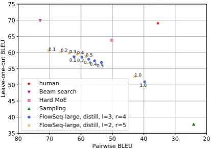
Following (Shen et al., 2019), we analyze the output diversity of FlowSeq. Shen et al. (2019) proposed pairwise-BLEU and BLEU computed in a leave-one-out manner to calibrate the diversity and quality of translation hypotheses. A lower pairwise-BLEU score implies a more diverse hy-pothesis set. And a higher BLEU score implies a better translation quality. We experiment on a subset of test set of WMT14-ENDE with ten references each sentence (Ott et al., 2018). In Fig. 6, we compare FlowSeq with other
multi-Figure 6: Comparisons of FlowSeq with human translations, beam search and sampling results of Transformer-base, and mixture-of-experts model (Hard MoE (Shen et al.,2019)) on the averaged leave-one-out BLEU score v.s pairwise-BLEU in descending order.
hypothesis generation methods (ten hypotheses each sentence) to analyze how well the genera-tion outputs of FlowSeq are in terms of diversity and quality. The right corner area of the figure in-dicates the ideal generations: high diversity and high quality. While FlowSeq still lags behind the autoregressive generations, by increasing the sam-pling temperature it provides a way of generating more diverse outputs while keeping the translation quality almost unchanged. More analysis of trans-lation outputs and detailed results are provided in the AppendixDandE.
5 Conclusion
We propose FlowSeq, an efficient and effective model for non-autoregressive sequence generation by using generative flows. One potential direc-tion for future work is to leverage iterative refine-ment techniques such as masked language models to further improve translation quality. Another ex-citing direction is to, theoretically and empirically, investigate the latent space in FlowSeq, hence pro-viding deep insights of the model, even enhancing controllable text generation.
Acknowledgments
[image:9.595.313.520.64.210.2]References
Dzmitry Bahdanau, Kyunghyun Cho, and Yoshua Ben-gio. 2015. Neural machine translation by jointly learning to align and translate. In International Con-ference on Learning Representations (ICLR).
Samuel R Bowman, Luke Vilnis, Oriol Vinyals, An-drew M Dai, Rafal Jozefowicz, and Samy Ben-gio. 2015. Generating sentences from a continuous space. arXiv preprint arXiv:1511.06349.
Yuri Burda, Roger Grosse, and Ruslan Salakhutdinov. 2015. Importance weighted autoencoders. arXiv preprint arXiv:1509.00519.
Jacob Devlin, Ming-Wei Chang, Kenton Lee, and Kristina Toutanova. 2018. Bert: Pre-training of deep bidirectional transformers for language understand-ing. arXiv preprint arXiv:1810.04805.
Laurent Dinh, Jascha Sohl-Dickstein, and Samy Ben-gio. 2016. Density estimation using real nvp. arXiv preprint arXiv:1605.08803.
Marjan Ghazvininejad, Omer Levy, Yinhan Liu, and Luke Zettlemoyer. 2019. Constant-time machine translation with conditional masked language mod-els. arXiv preprint arXiv:1904.09324.
Jiatao Gu, James Bradbury, Caiming Xiong, Victor OK Li, and Richard Socher. 2018. Non-autoregressive neural machine translation. In International Confer-ence on Learning Representations (ICLR).
Jiatao Gu, Qi Liu, and Kyunghyun Cho. 2019. Insertion-based decoding with automatically inferred generation order. arXiv preprint arXiv:1902.01370.
Sergey Ioffe and Christian Szegedy. 2015. Batch nor-malization: Accelerating deep network training by reducing internal covariate shift. In International Conference on Machine Learning, pages 448–456.
Diederik P Kingma and Jimmy Ba. 2014. Adam: A method for stochastic optimization. arXiv preprint arXiv:1412.6980.
Diederik P Kingma, Tim Salimans, Rafal Jozefowicz, Xi Chen, Ilya Sutskever, and Max Welling. 2016. Improving variational inference with inverse autore-gressive flow.The 29th Conference on Neural Infor-mation Processing Systems.
Durk P Kingma and Prafulla Dhariwal. 2018. Glow: Generative flow with invertible 1x1 convolutions. InAdvances in Neural Information Processing Sys-tems, pages 10215–10224.
Jason Lee, Elman Mansimov, and Kyunghyun Cho. 2018. Deterministic non-autoregressive neural se-quence modeling by iterative refinement. In Pro-ceedings of the 2018 Conference on Empirical Meth-ods in Natural Language Processing, pages 1173– 1182.
Jindˇrich Libovick`y and Jindˇrich Helcl. 2018. End-to-end non-autoregressive neural machine translation with connectionist temporal classification. In Pro-ceedings of the 2018 Conference on Empirical Meth-ods in Natural Language Processing, pages 3016– 3021.
Xuezhe Ma and Eduard Hovy. 2019. Macow: Masked convolutional generative flow. arXiv preprint arXiv:1902.04208.
Xuezhe Ma, Zecong Hu, Jingzhou Liu, Nanyun Peng, Graham Neubig, and Eduard Hovy. 2018. Stack-pointer networks for dependency parsing. In Pro-ceedings of the 56th Annual Meeting of the Associa-tion for ComputaAssocia-tional Linguistics (Volume 1: Long Papers), pages 1403–1414.
Xuezhe Ma, Chunting Zhou, and Eduard Hovy. 2019. Mae: Mutual posterior-divergence regularization for variational autoencoders. InProceedings of the 7th International Conference on Learning Representa-tions (ICLR-2019), New Orleans, Louisiana, USA. Oren Melamud, Jacob Goldberger, and Ido Dagan.
2016. context2vec: Learning generic context em-bedding with bidirectional LSTM. InProceedings of The 20th SIGNLL Conference on Computational Natural Language Learning, pages 51–61, Berlin, Germany. Association for Computational Linguis-tics.
Myle Ott, Michael Auli, David Grangier, et al. 2018. Analyzing uncertainty in neural machine translation. In International Conference on Machine Learning, pages 3953–3962.
Myle Ott, Sergey Edunov, Alexei Baevski, Angela Fan, Sam Gross, Nathan Ng, David Grangier, and Michael Auli. 2019. fairseq: A fast, extensible toolkit for sequence modeling. In Proceedings of NAACL-HLT 2019: Demonstrations.
George Papamakarios, Theo Pavlakou, and Iain Mur-ray. 2017. Masked autoregressive flow for density estimation. InAdvances in Neural Information Pro-cessing Systems, pages 2338–2347.
Ryan Prenger, Rafael Valle, and Bryan Catanzaro. 2019. Waveglow: A flow-based generative net-work for speech synthesis. In ICASSP 2019-2019 IEEE International Conference on Acous-tics, Speech and Signal Processing (ICASSP), pages 3617–3621. IEEE.
Danilo Jimenez Rezende and Shakir Mohamed. 2015. Variational inference with normalizing flows. In
Proceedings of the 32nd International Conference on International Conference on Machine Learning-Volume 37, pages 1530–1538. JMLR. org.
Tianxiao Shen, Myle Ott, Michael Auli, et al. 2019. Mixture models for diverse machine translation: Tricks of the trade. InInternational Conference on Machine Learning, pages 5719–5728.
Raphael Shu, Jason Lee, Hideki Nakayama, and Kyunghyun Cho. 2019. Latent-variable non-autoregressive neural machine translation with de-terministic inference using a delta posterior. arXiv preprint arXiv:1908.07181.
Mitchell Stern, William Chan, Jamie Kiros, and Jakob Uszkoreit. 2019. Insertion transformer: Flexible se-quence generation via insertion operations. arXiv preprint arXiv:1902.03249.
Ashish Vaswani, Noam Shazeer, Niki Parmar, Jakob Uszkoreit, Llion Jones, Aidan N Gomez, Łukasz Kaiser, and Illia Polosukhin. 2017. Attention is all you need. InAdvances in neural information pro-cessing systems, pages 5998–6008.
Oriol Vinyals, Alexander Toshev, Samy Bengio, and Dumitru Erhan. 2015. Show and tell: A neural im-age caption generator. In Proceedings of the IEEE conference on computer vision and pattern recogni-tion, pages 3156–3164.
Martin J Wainwright, Michael I Jordan, et al. 2008. Graphical models, exponential families, and varia-tional inference. Foundations and TrendsR in
Ma-chine Learning, 1(1–2):1–305.
Yiren Wang, Fei Tian, Di He, Tao Qin, ChengXiang Zhai, and Tie-Yan Liu. 2019. Non-autoregressive machine translation with auxiliary regularization.
arXiv preprint arXiv:1902.10245.