Abstract—A modified genetic algorithm (GA) is presented for
subsonic wing design using an N-S flow solver with B-L turbulence model. With the feature of revolution in-subsection, the algorithm takes advantage of binary coding system, and overcomes the large search space problem of requiring continuous sampling. The modified genetic algorithm remarkably improves computational efficiency by coupling with robustness, crossing-over and mutation operators. The resulting optimized subsonic wing has a higher lift-drag ratio than the initial shapes do. By this optimal design method, the algorithm introduced more parameters (twisted angles) for aerodynamic configuration design, and thus demonstrates better of feasibility, robustness, and design outcome for subsonic wing configuration. The resulting outcomes confirm that the method shows quicker in convergence, in comparison to the traditional genetic algorithms.
Index Terms—Genetic algorithm, revolution in-subsection,
twisted angle, plane shape
I. INTRODUCTION
Aerodynamic design can be defined as a process determining the shape of bodies in order to satisfy a design aim and the associated constraints, in terms of aerodynamics, geometry or structure. The design aim of aerodynamics is to obtain a vehicle configuration with optimal performance, and thus the configuration has a much higher lift-drag ratio than conventional vehicle geometries. . In other words, a design must meet several criteria at a certain cruising speed with designed lift coefficients and desired drag characteristics. A variety of optimal methods in Computational Fluid Dynamics (CFD) are used more and more for vehicle design. The optimal methods in the aerodynamic design can obviously reduce the time of design cycle. Meanwhile, the rapid improvement of computer capabilities has made various numeric-optimal techniques available in the application of aerodynamic design. The techniques take account of the matured gradient, automatic differentiation, Adjoint-Based method, and genetic algorithms [2-5,8,9] (GA). When the optimal methods are in use, however, we need consider:
Manuscript received March. 4, 2008
Sun Gang, Mechanics and Engineering Science Dep., Fudan Univ., Shanghai 200233, China, Tel: 0086-21-65642740,Fax: 0086-21-65642742; email:[email protected];
Chen YingChun, The first aircraft institute of China, ShangHai 200232,China. [email protected]
Alex H. Leo, Baker University, 8001 College Blvd., Suite 100, Overland Park, KS 66210, USA, email: [email protected] )
a) The general applicability of the optimal formulation immediately for different application problems, including also the usage of different analysis tools. b) The robustness, the capability intended to find global
optimization and reduction of the interaction between human and expert knowledge.
c) The ability to deal with multiple design objectives and constraints.
d) The Computational efficiency in the practical application of a design approach.
The GA is in possession of different advantages in optimal fitness. By binary coding system for the fitness, the traditional optimal algorithm can inherently carry out the crossover and mutation operations, and completely make the use of implicit parallel quality. But, when the number of parameters and the required precision are in high degree, the length of the binary-code string becomes so long, that the searching efficiency of GA algorithm is dropping, and in consequence, that the global optimization efficiency of GA is impaired.
The purpose of this paper is to improve the performances of GA, through introducing an approach, ‘subsection evolution’, which divides the whole evolutional progress into two subsections. In the first one, the length of a binary-code string is set to a properly designated value in advance for improving the searching efficiency for a temporary optimal fitness. Based on it, a genetic optimization for high precision is executed in the second subsection. Coupled with the robust crossover and mutation operators, the approach behaves more efficient than before. In comparison to the initial shapes, the resulting optimal airfoil and wing have a higher lift-drag ratio, and reveals the feasibility and robustness of this newly designed optimization method.
II. EVOLUTIONARY GENETIC ALGORITHM IN SUBSECTION A.Binary Representation
For the designing of wing by means of binary genetic optimized coding, it is proper to assume a multi-dimensional function defined as:
} , . 2 , 1 ], , [ | ) , , , (
max{f x1 x2L xn xi∈ ui vi i= Ln
(1) And then mapping the dorman [ui, vi] of an undependable variable (xi) into [0,1] interval is as following:
]
1
,
0
[
]
,
[
u
iv
i→
i
n
u
v
u
x
x
x
i i
i i i
i
−
=
1
,
2
,
L
,
−
=
′
→
(2)An Optimal Design for Subsonic Wing Planar
Shape and Twisted Angle by a Modified Genetic
Algorithm
So that xi could be presented as a binary form and determined in length. Given the precision of wing designing as 10–t, and set
n
i i i
m
v
u
d
1}
max{
=−
=
as the upper boundary of the domains of the independent variables, dm is used to define the binary coding length throughout the genetic evolution algorithm cooperatively with the set precision 10-t. Therefore, the length (m-bit) for the binary coding is defined by the following equation:
m t m m
d
10
2
2
−1≤
⋅
≤
So far, a chromosome bi comes and B is a vector of the (n) chromosomes, described as a binary string in m-bit.
[
b
b
n]
B
=
1L
Where
im i i
i
b
b
b
b
=
1 2L
Through a genetic evolution algorithm, the resulting optimized (n) variables are all as following
1
2
2
)
(
1 0 ,−
−
+
=
∑
− = − m m j j j m i i i i ib
u
v
u
x
(3)In order to express Mutation Operator evidently, a normalizing process is used in binary code. But the normalization results in the following faults:
(1) It asks that Genetic coding has same expression and range. Although it has the advantage with binary coding, it has a longer Hamming distance between neighbored codes. For example, the binary codes of 15 and 16 are 01111 and 10000 respectively, and the algorithm searching from 15 to 16 needs modify all five bits of binary code. It is very time-consuming to do so with crossover and mutation operators. This denotes both a longer time for fitting and a higher risk falling into a local optimal trap in the searching. This is the Hamming problem of binary coding.
(2) When the high precision is in place, the expression of a binary code is very redundant, which will reduce searching efficiency.
The solution of creep mutation is introduced to solve the Hamming problem. The principle is to set 1 whether added to or subtracted from a binary number for genetic code in the Hamming problem.
The idea of subsection evolution is introduced to improve the searching efficiency. The evolution of resulting generation consist of the following steps:
Step 1: given (n) initial binary variables in (m + k)-bit, the binary bits of a variable are divided into two substrings in m- and k-bit respectively;
Step 2: the substrings in m-bit are considered. Fed into the genetic algorithm, the (n) substrings in (m)-bit evolve into (n) resulting-optimized strings, x*, in (m)-bit; Step 3: make every substring in (k)-bit into in (k+1)-bit by
entailing an extra bit;
Step 4: feeding these new entailed substrings in (k+1)-bit to the algorithm come (n) strings in (k+1)-bit;
Step 5: following the first (m-1) bits of the substring x*, a new resulting substring in (k+1)-bit becomes into
(m+k)-bit;
Step 6: feeding the resulting string in (m+k)-bit to the genetic algorithm over again, comes a temporary optimal string;
Step 7: combining the first (m-1) bits of the substring x* and the last (k+1) bits of the temporary sub-string together, the (n) optimized substrings become in (m+k)-bit finally.
The above seven steps of evolution result in a generation, and each and every generation comes in the same way by the evolution. It is available to prove that optimal variable approaches at the required-precision level.
In accordance with the above description, by means of decoding and mapping, the expressed original value of the (m + k)-bit of i th string is:
∑
+ − = + − + +−
−
+
=
1 02
1
2
k m j j j k m k m i i i k m ib
u
v
u
x
(4)In the subsection evolution, the expression of combing the substring in m-bit and substring in k–bit is:
⎥ ⎥ ⎥ ⎥ ⎦ ⎤ ⎢ ⎢ ⎢ ⎢ ⎣ ⎡ − + − − + = + − = +− − = − ⋅
∑
∑
1 2 2 1 2 2 ) ( 1 0 1 0 k m k j j j k m m m j j j m i i i k m i b b u v ux (5)
Subtracting the above two expressions come the following:
) 2 2 )( 1 2 ( 2 1 2 ) ( 1 0 k m m k m j j j m i i k m i k m
i x v u b
x − − − = − + ⋅ − − − ⋅ ⎟⎟ ⎠ ⎞ ⎜⎜ ⎝ ⎛ − =
−
∑
(6)And ) 1 2 ( − − < − + ⋅ m i i k m i k m i u v x
x (7)
In an evolution, the maximum error of a string in (m+k)-bit, a substring in m-bit entailing a substring in k-bit, is less than a weighted value of the first (m) bits of the initial string. In Steps 1 and 2, the first (m-1) bits of the resulting substring in m-bit are the first part of the final accurate value. Since and after Step 3, through the evolving of the substring in (k+1)-bit and being entailed, a final string in (m+k)-bit becomes the value in high precision. Thus, the fitness is available to calculate according to the formula (4). As the GA is for the multi-dimensional optimization or high precision fitness, the variables have to be binary strings. And if they are of long form, the subsection evolution is a choice to avoid low efficient searching.
B. Genetic operators
The Genetic operators are of the following three steps: (1) Selection and reproduction
Parents are chosen based on the Roulette-wheel method, in which the probability of choosing a parent is proportional to its fitness value. Each pair of parents produces one offspring by crossover. Then, Mutation occurs in the offspring. After a new population is produced, the fitness of each member is compared to that of the parent generation, and the best and the second best members in the new born generation are assigned as the new parent generation, and strike away the inferior crossover or mutation. This technique in use guarantees that the best member in all the populations will not be screened out by means of the GA operators during the optimal procedure.
The uniform crossover scheme [6] takes place in the present paper. Based on the uniform probability, it is determined how to substitute every genetic bit of a parent. The crossing is not in place at a genetic bit where it is equal to 0, and but as it is equal to 1. The crossing appears as follows:
[
]
[
]
[
]
⎩⎨[
[
]
]
⎧⇒ →
⎭ ⎬ ⎫
00110101 11101010 10011100
10101001 01110110
crossover
Mutation[7] is carried out by randomly selecting a gene (geometric node) and then changing its value randomly within a preset range. As this change is applied to the selected geometric node, the neighbors of the node are so adjusted that the curvature of the sectioned profile is not over-abrupt.
(3) Replication
An elite-preservative operator is used for replication as parental binary strings in the present paper. The mechanism of the survival of the fittest guarantees the best individual of the current generation to be replicated into next generation. The mechanism is to check if the best individual of parent is preserved when the new generation is born. As not so, a random chosen individual in gene takes place from the parent generation. Experimental results proved that this mechanism would effectively prevent the optimal chromosomes from losing.
III. COMPUTATION FLUID DYNAMICSOLVER
In terms of CFD-based performance assessment, a fluid-oriented solver [1] based on B-L turbulent model, is in use for the viscid fluid of subsonic airfoil and wing. Once the designing variables are set by the GA, the solver has to be called in by feeding the designing variables into it. The solver then yields the ratios of lift-to-drag. These values are then stored up in a file. They can be used by the GA for the calculation of the optimal objective and hence the fitness functions. For an individual in a generation, at least once CFD call is needed. Therefore, an enormous number of CFD calls are necessary for the entire optimization.
IV. PERFORMANCE TEST OF THE ALGORITHM A multi-modality function comes to test the performance of the subsection-evolution GA operator:
) 64 . / ) 0667 . ( 2 log 4 . exp(
) 5 . 0 ) .) 1 tan( 0 . 4 1 . 5 (sin(
) 64 . / ) 0667 . ( 2 log 4 . exp(
) 5 . 0 ) .) 1 tan( 0 . 4 1 . 5 (sin(
2 6 2
6
− ⋅ ⋅ −
⋅ + ⋅ ⋅
⋅ ⋅
− ⋅ ⋅ −
⋅ + ⋅ ⋅
⋅ =
y y da
x x da
[image:3.612.335.525.94.251.2]f
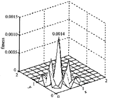
Fig. 1 shows the spatial structure of the multi-modality function. The maximum value is the optimal objective. The constraint condition is x y, ∈[0.0, 2.0]. It is evident that the achieving of maximum may well be prevented from the maximum by trapping in a local maximum. David L. Carroll[5] chose binary code for GA operator in 2001,the population number as 5, and the fitness value of function. Fig. 2 shows results of the compare off-line performance between the initial GA model and optimized GA model. The horizontal axis expresses the evolution generation,the vertical axis expresses the optimal fitness value of every generation. The global optimal value is achieved at generation 20 with
optimized GA model, yet at generation 50 with the initial GA. It shows that the searching performance of optimized GA model is in excess the initial GA model.
[image:3.612.324.529.125.458.2]Fig.1 2-dimensional multimodality function
Fig.2 Comparison of off-line performance between initial GA and optimal GA
V. RESULTS AND DISCUSSION A. Optimization of Airfoil
The GA works on designing variables subject to certain performance constraints. A Hicks-Henne function curve is used to represent airfoil. The actual values of (x, y) coordinates of the control nodes for the B-spline curves are set as the designing variables
0
1
( )
( )
( )
n
k k k
y x
y x
c f x
=
=
+
∑
. Where Hicks-Henne function
0.25 20
3 ( )
(1 ) , 1
( )
sin ( ) , 1
x
k e k
x x e k
f x
x k
π
−
⎧ − =
⎪
= ⎨ >
⎪⎩
( )
lg 0.5 / lg
k,0
1
e k
=
x
≤ ≤
x
The NACA0012 airfoil is used to test the present algorithm for initial airfoil shape. The N-S equations are associated with B-L turbulent model for field simulation. Lift-to-drag ratio of airfoil is as fitness:
d l C
C
[image:3.612.326.529.286.467.2]The free stream of fluid is:
0
5 . 6 , 28 .
0 =
=
∞ α
M .
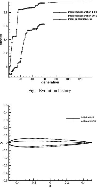
[image:4.612.325.525.68.455.2]For satisfying structural requirements of aircraft, the constraint condition of airfoil is: the thickness of airfoil limits in 0.04~0.12. Table 1 shows the outcomes of lift, drag and lift-to-drag ratio of the initial vs. optimized value. Through 60 iterations, it shows that optimized drag declines and the lift-to-drag ration increase about 9.9% with the initial GA, 14.19% with the optimized GA, as well as the outcomes of high aerodynamic performance. Fig.3 shows that the mesh distribution of the airfoil. The convergent history of the
Fig.3 Mesh distribution of airfoil
[image:4.612.100.271.192.352.2]computation is shown in Fig. 4. In comparison to the initial GA, which does not get the converged after 60 CFD calls, while the subsection evolution optimized GA get converged after 60 CFD calls, reaching the fitness. So to speak, the improved evolutional method performs in quality for convergence. The best of fitness is of the best individual member of each generation, though the other fitness are related to the non-best members. The trend of the fitness in fig. 4 clearly shows that the optimization is the approaching of generation-by-generation, and the reliability of the subsection evolution GA. Fig.5 shows the designed optimal airfoil in comparison to the initial one. The designed shape demonstrates the modifying through from the leading edge to the trailing edge of the airfoil.
Table 1 Aerodynamic property comparison between GA vs. GA modified
Coeff. initial GA GA Modified
l
C 0.830094 0.828735 0.827376
d
C 0.105782 0.096055 0.092365
/
l d
C C 7.847208 8.627700 8.957582
generation
fi
tn
e
ss
20 40 60 80 100 120
8 8.2 8.4 8.6
8.8 improved generation 1-60
improved generation 60-140 initial generation 1-60
Fig.4 Evolution history
x
y
-0.4 -0.2 0 0.2 0.4
-0.5 -0.4 -0.3 -0.2 -0.1 0 0.1 0.2 0.3 0.4 0.5
initial airfoil optimal airfoil
Fig.5 Comparison of initial vs. optimized airfoil
B. Optimization of Wing Planar Shape
In wing configuration design, the airfoil’s formula is determined. The mesh distribution of a wing chooses the C-H configuration. The C mesh is distributed along the streamline direction and the H mesh is distribution along the span direction. The planar parameters of a wing are to be optimized. They include the wing sweep, root chord, span, and tip chord. The planar constraint conditions of the wing are [0.3491, 0.6982], [0.8, 1.0], [1.0, 1.2] and [0.4, 0.5] respectively; the constraint condition of airfoil is: the thickness is limited within 0.04~0.12. There are all 18 such optimal parameters, including 14 parameters for airfoil design and 4 parameters for wing plane design. The maximum evolution number is set at 70; the population number of the first 30 generations is set at 10; the number of the rest 40 generations is set at 5. The free stream condition is:
0
5 . 4 6 .
0 =
=
∞ α
M
[image:4.612.86.287.589.641.2]higher aerodynamic performance by means of the optimized GA.
Table2 Aerodynamic parameters comparison between initial and optimal wing shape Aerodynamic Initial Optimal
l
C 0.546503 1.446295
d
C 0.233342 0.388092
/ l d
C C 2.342066 3.726676
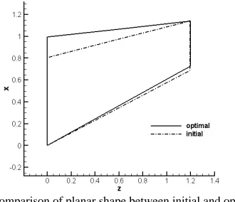
Table 3 shows the comparison of planar parameters between initial and optimized wings, increasing of the span, root chord and sweep, declining of the tip chord, as well as improvement in the aerodynamic performance of the wing.
Table3 Comparison of planar parameter value between initial and optimal wing Plane initial optimal
sweep 30 31.293414
Span 1.1963 1.1992
Root Chord 0.8059 0.9967 Tip chord 0.4533 0.4096
Fig. 8 shows the initial wing plane in comparison to the optimal wing plan. As table 3, the planar shape varies the chord and sweep respectively. Fig. 9 shows the optimal evolution history and the high optimal performance.
C Optimal of Wing twist angle
The root twisted and tip twisted angles are respectively considered as [-0.55,-0.50],[-0.08,-0.02] through the optimizing of parameters. Here are 20 optimized parameters totally, of which 14 for airfoil designing and 6 for wing plane designing. The maximum evolution number is at 70, the population number of the first 30 evolutions is set at 10, the following 40 evolutions is set at 5. The free stream condition is:
0
5 . 4 6 .
0 =
=
∞ α
M
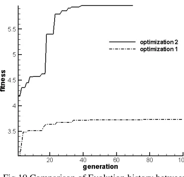
[image:5.612.347.512.585.727.2]Table 4 demonstrates, through 40 iterations, in terms of the lift, drag and lift-to-drag, the comparison of the optimized outcomes without twisted angle vs. those with twisted angle, optimized drag deducing, the lift-to-drag increasing up to about 60%, the resulting higher aerodynamic performance by the optimized GA, regarding the twisted angles of wing section as design parameters. Table 5 shows the comparison of planar parameters of a wing between optimal without twisted angular parameters and with. It shows that the span, root chord and sweep are increased, the tip chord and span are deduced, which change the aerodynamic performance of wing.
Fig.9 Evolution history Table 4 Aerodynamic property comparison
between optimization 1 and optimization 2 aerodynamic Optimal 1 Optimal 2
l
C 1.446295 0.960661
d
C 0.388092 0.161045
/ l d
[image:6.612.90.280.381.461.2]C C 3.726676 5.965172
Table 5 Comparison of planar parameter value between initial and optimal wing Planar initial design
sweep 30 39.348105
span 1.1963 1.1852
Root chord 0.8059 0.9829 Tip chord 0.4533 0.4385
Root twist 0 -0.516694
Tip twist 0 -0.037367
[image:6.612.89.274.541.719.2]Fig. 10 shows the evolution history of optimizing with twisted-angle parameter (optimization 1) and without (optimization 2). It also shows that the more wing parameters are chosen, the better aerodynamic result of a wing is obtained.
Fig.10 Comparison of Evolution history between optimization 1 and optimization 2
VI. SUMMARY
An approach, ‘subsection evolution’, dividing an entire evolution process into two subsections, with binary coding, coupled with the robust crossover and mutation operators, improves the original GA optimal efficiency greatly. Combined with the CFD solver in high precision and the optimized GA method for aerodynamic optimization, the resulting airfoil and wing has a higher lift-to-drag ratio than the initial shapes. The invented optimizing approach also demonstrates a great feasibility and robustness in engineering computation.
REFERENCES
[1] Jameson A Schmidt W and Turkel E. Numerical Solutions of the Euler Equations by Finite Volume Methods Using Runge-Kutta Time Stepping[R]. AIAA Paper 81-1259, June 1981.
[2] Goldberg J H. Genetic Algorithms in Search, Optimization and Machine Learning[M]. Addison-Wesely. Reading MA, 1989.
[3] Hicks R, Henne P. Wing Design by Numerical Optimization[J]. Journal of Aircraft, 1978, 15 (7): 407-413. [4] K. Krishnakumar, Micro-Genetic Algorithms for Stationary
and Non-Stationary Function Optimization[J]. Intelligent Control and Adaptive Systems, 1989, 1196. Philadelphia, PA. [5] D. L. Carroll, Genetic Algorithms and Optimizing Chemical Oxygen-Iodine Lasers[A]. ln: H. Wilson et al. Developments in Theoretical and Applied Mechanics, Vol. XVIII[C]. School of Engineering, The University of Alabama, 1996. 411-424. [6] G. Syswerda, Uniform Crossover in Genetic Algorithms [A].
The Third International Conference on Genetic Algorithms[C].
[7] Morgan Kaufmann, Los Altos, California, 1989. 2-9.V. Coverstone-Carroll, Near-Optimal Low-Thrust Trajectories via Micro-Genetic Algorithms[J]. Engineering Notes, 1997, 20: 196-19
[8] WANG Xiao-peng. Study of Genetic Algorithm and Its Use in Aerodynamic Optimization Design[D]. Northwestern Polytechnical University, 2000.