Abstract— Parameter estimation technique is an indispensable computational tool not only in aerospace research activities but also industrial activities such as control law design, handling qualities evaluation, model validation, and flight-vehicle design and certification. The estimation methods yield different levels of associated error with the estimated parameters. The primary reason for this is linked to the presence of measurement and process noise with the real flight data. Equation Error Method cannot handle either process noise or measurement noise. Output Error Method can handle measurement noise but not process noise. Filter Error Method, a special case of Output Error method, can be advantageously used to estimate parameter from flight data having both process and measurement noise. This paper presents issues related to the application of FEM with Gauss Newton (GN) and Levenberg-Marquardt (LM) optimization in estimating aerodynamic parameters from in-house generated flight data.
Index Terms—Parameter Estimation, Equation Error Method, Output Error Method, Filter Error Method
I. INTRODUCTION
Since mid-sixties the field of system identification has developed into an indispensible tool with application to engineering systems like aerospace vehicles. One of the first definitions of system identification was given by Zadeh[1] : “Identification is the determination, on the basis of input and output, of a system within a specified class of systems to which the system under test is equivalent”. Broadly speaking, system identification, as it is termed today, is a scientific discipline which provides answer to the age-old inverse problem of obtaining a description in some suitable form for a system given its behavior as a set of observations [2]-[3]. There are three elements essential to a system identification problem, a system (model), an experiment and a response (output or measurement). The most widely applied subfield of system identification is the filed of parameter identification wherein an assumed mathematical model based on the phenomenological considerations is used to estimate the properties of the dynamic system [3]-[4]. The model contains a finite number of parameters, the values of which must be deduced from measured data. The assumed model,
Manuscript submitted December 29, 2007.
1Phd Student, Department of Aerospace Engineering, Indian Institute of Technology Kanpur, India, email: [email protected], Phone: +91 (0512)2597716
2P.G. Student, Department of Aerospace Engineering, Indian Institute of Technology Kanpur, India, [email protected], Phone: +91 (0512)2597716 3Associate Professor, Department of Aerospace Engineering, Indian Institute of Technology Kanpur, India, [email protected], Phone: +91 (0512)2597716
however, will not be an exact representation of the system, no matter how careful its selection is. Furthermore, the experimental data made with real, and thus imperfect instruments will not be consistent with the assumed model form for identified values of system parameters. So the revised task of determining the best estimates, rather than the exact values of the parameters is more properly called parameter estimation. The two most important sub-problems of parameter estimation are: the definition of the criteria for the best, and the characterization of potential errors in the estimation.
Aircraft parameter estimation is probably the most outstanding and illustrated example of the system identification methodology: The highly successful application of system identification to flight vehicle has been possible partly due to better measurement techniques and data processing capabilities provided by the digital computers, partly due to the ingenuity of engineers in advantageously using the developments in other fields such as estimation and control theory, and partly due to fairly well- understood basic physical principles leading to adequate aerodynamic modeling, and design of appropriate flight tests [4]-[6]. The equations of motion of flight vehicle are derived from Newtonian Mechanics [7]-[8], usually assuming flight vehicle to be rigid body. The mathematical models based on such equations of motion assume that the forces and the moments acting on the flight vehicle can be synthesized. Out of the various forces and moments (aerodynamic, inertial, gravitational and propulsive) acting on a flight vehicle, it is the determination of the aerodynamic forces that poses the most difficult challenge till date. To a large extent, it is the adequacy and accuracy of modeling the aerodynamic forces and moments that would determine the validity and utility of the mathematical models.
After a-priori fix of the model, the next task of estimating parameters (stability and control derivatives) has been attempted by three different but complimentary techniques: analytical methods, wind-tunnel methods and flight test methods. At initial stages of aircraft design, analytical methods [9]-[11] provide the only convenient way of estimating the aircraft parameters. However the accuracy of such theoretical estimates being not so high, there is a need to verify these estimates with those obtained from wind-tunnel testing and flight tests. Although wind-tunnel methods improve the accuracy of estimation of parameters, they are time consuming and expensive. Furthermore, simulation of control surfaces, power effects and stringent flight conditions are difficult to simulate satisfactorily. Wind-tunnel estimates also suffer from discrepancies due to interference effects of support systems, wall effects, turbulence level, etc. It is,
Aerodynamic Characterization of HANSA-3
aircraft using Equation Error, Maximum
Likelihood and Filter Error Methods
Naba Kumar Peyada1, Arpita Sen2 and Ajoy Kanti Ghosh3
therefore, desirable that the wind-tunnel estimates be validated against the estimates from flight test data.
Modern methods of aircraft parameter estimation can be broadly classified into three categories [2]: (i) Equation Error Methods (EEM), (ii) Output Error Methods (OEM) and (iii) Filter Error Methods (FEM). These methods belong to a class called “direct-approach”. Another approach wherein a nonlinear filter provides estimates of parameters which are artificially defined as additional state variables is sometimes referred to as “indirect-approach”. While the EEMs represent a linear estimation problem, the remaining methods belong to a class of nonlinear estimation problems. The EEMs and OEMs are deterministic methods, as opposed to the stochastic approach of FEMs. The EEMs are based on linear regression using ordinary least squares technique. Its main advantage lies in its computational simplicity and non-iterative nature. However in presence of measurement noise, the least square estimates are asymptotically biased, inconsistent and inefficient [5]. The OEM is probably the most frequently used method for aircraft parameter estimation. The OEMs search for those values of parameters that minimize the error between flight measured responses and corresponding responses of the assumed mathematical model. Various aspects of the OEM approach and its most employed version, the Maximum Likelihood (ML) Method, are well documented by Maine and Iliff [5]. The main advantage of the ML Method is that the parameter estimates are asymptotically unbiased, consistent and efficient. The method also provides a measure of accuracy in terms of Standard Deviation as in the computations in this paper [5]. The ML estimates of model parameters accounting only for measurement noise can be effectively used for linear and general nonlinear systems [12]. In the presence of atmospheric turbulence, the OEM yields poor results.
Accuracy of parameter estimates is directly dependent on the quality of the flight data and hence (i) it requires highly accurate measurements of control and motion variables (ii) the maneuvers should be carried out under calm atmospheric conditions. Both these above requirements are difficult to meet practically. The measurement error can be minimized by appropriate selection of sensors and by following dedicated sensor calibrations. However, it is generally difficult to completely account for the turbulence through a-priori modeling. FEM in such situations can advantageously be applied. FEM is perhaps the most general stochastic approach to aircraft parameter estimation [12], which accounts for both process and measurement noise and was proposed by Balakrishnan [13].
In the present work, parameter estimation exercise has been carried out by applying EEM, ML method of OEM, and FEM on measured longitudinal flight data. The flight data has been generated by carrying out longitudinal maneuvers using in-house HANSA-3 [14]aircraft.
II. GENERATIONOFFLIGHTDATA
The proposed method is investigated using real flight data (longitudinal mode) generated using research aircraft (HANSA-3) available with Indian Institute of Technology Kanpur [14], a research aircraft designed and developed by National Aerospace Laboratories (NAL), India.
A flight data base for identification studies was gathered from flight maneuvers with the test aircraft. Typically, starting from trim flight conditions, the pilot applied control input in an attempt to excite the chosen dynamic modes. An onboard measurement system installed in the research aircraft measured
V
, , , , , ,
α θ
q a a
z xδ
e. The measurement of airspeed( )
V , angle of attack (α
) were obtained with flight log mounted on a boom fixed to the tip of the wing. The angular rateq
was obtained from the measurements available from the inertial platform. The accelerations along the three body axes were measured using an accelerometer triad located near the CG of the aircraft. The rate of angular rateq
&
was obtained by numerical differentiation ofq
. The control surface deflectionδ
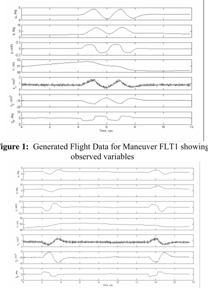
e was measured using potentiometer. The temperature T was recorded using the standard cockpit outside air temperature (OAT) gauge. Two sets of flight data simulating short period longitudinal dynamics were generated at an altitude 6000 feet. The cruise speed at which the perturbations were initiated was fixed at nearly 56 m/s.The longitudinal flight data (FLT1) was generated using multi step elevator input
(
δemax=7deg)
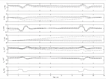
having total duration of 4s only. Another flight data set (FLT2) was generated with two similar looking double pulse input having almost same magnitude. These two pulses although look similar but have opposite elevator deflection to excite the longitudinal dynamics. In this paper two sets of flight data (FLT1 and FLT2) having input application during of 4 and 2s are considered for analysis and investigation. The acquired flight data (FLT1 and FLT2) are presented in Fig. 1 and Fig. 2.Figure 1: Generated Flight Data for Maneuver FLT1 showing observed variables
[image:2.612.325.533.421.709.2]III. EQUATIONSOFMOTIONANDAERODYNAMICMODEL The aerodynamic derivative in the wind axis system (lift and drag derivatives) are obtained through standard axes transformation from body axis non-dimensional derivatives
x
C and Cz. So for the longitudinal parameter estimation the following wind axis model has been used [8], [12].
(
)
D sin(
)
(
e)
cosV&= −qS m C +g α θ− + F m α
(1)
(
qS mV C)
L q(
g V) (
cos) (
F mVe)
sinα&= − + + α θ− − α(2) q
θ =&
(3)
(
y)
m(
e y)
tzq&= qSc I C + F I l
(4) Where, the lift, drag and pitching moment coefficients are model in Eq. (5-7).
0 e
D D D D e
C =C +C αα+C δ δ (5)
(
)
0 q 2 e
L L L L L e
C =C +Cαα+C qc V +C δ δ (6)
(
)
0 q 2 e
CG
m m m m m e
C =C +C αα+C qc V +C δ δ
(7) The longitudinal and vertical force coefficients CXand
Z
C are given in Eq.(8-9).
sin cos
X L D
C =C α−C α (8)
cos sin
Z L D
C = −C α−C α (9)
X z
C and C are calculated as per in Eq.(10-11)
(
cos)
/CG
X x eng eng
C = ma −F σ qS (10)
(
sin)
/CG
Z z eng eng
C = ma +F σ qS (11) So for the longitudinal case the unknown system parameter, which have to be estimated are given in Eq. (12)
0 e 0 q e 0 q e
T
D D D L L L L m m m m
C Cα Cδ C Cα C Cδ C Cα C Cδ
⎡ ⎤
Θ =⎣ ⎦ (12)
During the parameter estimation using the above postulated model described in Eqs. (5-7) V, ,α θand qare considered as state variables. The process noise is influenced by the process or state variable. So, the initial process noise matrix is the maximum difference of the measured data of , ,V α θandq. The element of process noise matrix is dependent on corresponding state variables.
IV. METHODSOFDATAANALYSIS
The various parameter estimation methods can be broadly classified into three categories [2]: i) Equation Error Methods (EEM) ii) Output Error Methods (OEM) iii) Filter Error Methods (FEM).
A. Equation Error Method
At any time
t
k, the dependent variablesy
(
t
)
can be expressed in terms of the independent variablesx
(
t
)
as,( )
( )
( )
( ) ( )
i 1 1 2 2
y k =θX k +θ X k + ⋅⋅⋅⋅ +θnXn k +ε k ; k=1, 2,⋅⋅⋅N ……..(13) Where
ε
denotes the stochastic equation error.Also,
θ
=
[
θ
1 T n]
...
2
θ
θ
denotes the vector of unknown parameters (the unknown stability and control derivatives to be estimated).The equation (13)can be represented in matrix notation as
( )
T( )
( )
y k =X k θ ε+ k (14)
So for N discrete time points we can prepare a matrix notation like
Y=Xθ ε+ (15)
Y
andε
areN
×
1
size vectors andX
is the qN n
×
matrix of independent variables:1 2 1 2 1 2 1 2 (1) (1) (1)
(2) (2) (2)
(3) (3) (3)
( ) ( ) ( ) nq nq nq nq x x x
x x x
X x x x
x N
x N x N
⎛ ⎞ ⎜ ⎟ ⎜ ⎟ ⎜ ⎟ = ⎜ ⎟ ⎜ ⎟ ⎜ ⎟ ⎜ ⎟ ⎝ ⎠ L L L L L L L L (16)
Equation error is given by Y X
ε= − θ (17)
Then by minimizing sum of the squares of the residuals, we shall arrive at the desired parameters. The cost function is defined as
( )
1 2 TJ θ = ε ε (18)
For minimum error, ( ) 0 J θ θ ∂ = ∂ (19)
From which we obtain the normal equation:
(
)
1ˆ X XT X YT
θ= − (20)
Equation (20) is our required working equation, where
[
1 qc/2V e]
X= α δ (21)
[
DC C
L m]
Y
=
C
(22) B. Output Error MethodCalculation of values of parameters in this case was done with maximum Likelihood (ML) method, a variant of OEM. Equations of motion of aircraft in state space are given by the equations [2]:
0 0
( )
( )
( )
x,
( )
x t
&
=
Ax t
+
Bu t
+
b
x t
=
x
(23)( )
( )
( )
yy t
=
Cx t
+
Du t
+
b
(24)( )
( )
( )
z k
=
y k
+
ν
k
(25) Wherex
andy
are the state and observation vectors respectively andu
is the control input.A B C
, ,
andD
are the matrices containing the unknown parameters, andz
is the measured variable, withν
being the measurement noise matrix.Estimates of parameter vector
θ
=
[
θ
1 T n]
...
2
θ
θ
isobtained on minimizing cost function
[
]
1[
]
1 2
1
( , ) N ( ) ( ) T ( ) ( )
k k k k
k
J R z t y t R− z t y t
=
Θ =
∑
− % − % (26)Where
R
is the measurement noise covariance matrix, given by[
][
]
1
1 N ( ) ( ) ( ) ( ) T k
R z k y k z k y k N =
=
∑
− − (27) Wherey k
( )
is the measured variable andz k
( )
is the observed variable for any timet
k.Updation of parameters is given by Gauss Newton formulation
1
, and
i+ i
Where
1 1
( ) T ( )
N
k
y t y t k R− k
=
∂ ∂
⎡ ⎤ ⎡ ⎤
= ⎢ ∂Θ ⎥ ⎢ ∂Θ ⎥
⎢ ⎥ ⎢ ⎥
⎣ ⎦ ⎣ ⎦
∑
% %F (29) And
[
]
1 1 ( ) ( ) ( ) T N k k k y tk R− z t y t =
∂
⎡ ⎤
− ⎢ ∂Θ ⎥ −
⎢ ⎥
⎣ ⎦
∑
% %=
G (30)
C. Filter Error Method
The mathematical model of nonlinear system in state space is given by the stochastic equations [12], [15]:
[
]
0 0( )
( ), ( ),
( ),
( )
x t
&
=
f x t u t
β
+
Fw t
x t
=
x
(31)[
]
( )
( ), ( ),
y t
=
g x t u t
β
(32)( )
k( )
k( )
kz t
=
y t
+
Gv t
(33)Where
f
andg
are then
xandn
y dimensional general nonlinear real valued vector functionsPrediction step
( )
( )
1 1 0 0ˆ
(
)
( )
, ( ),
,
ˆ
k k tk k t k k
x t
x t
f x t
u t
dt
x t
x
β
+ +=
+
⎡
⎣
⎤
⎦
=
∫
%
(34)[
]
( )
k( ), ( ),
k ky t
%
=
g x t
%
u t
β
(35)Correction step
( )
( )
( )
( )
ˆ
k k k kx t
=
x t
%
+
K z t
⎡
⎣
−
y t
%
⎤
⎦
(36)The steady state Kalman gain matrix K is 1
T
K
=
PC R
− (37)Thecovariance matrix of the state prediction error, P, is obtained by solving a Riccati equation.
1
1
0
T T T
t
AP
+
PA
−
ΔPC R CP
−+
FF
=
(38)According to definition, the residual error and covariance matrix of the residuals (R) between measured output and predicted output from the prediction step setting∂ ∂ =J/ R 0, are represented respectively as
[
][
]
1
1
N( )
( )
( )
( )
Tk
R
z k
y k
z k
y k
N
==
∑
−
−
(39)Where, the cost function J is defined as
[
]
1[
]
1 2
1
( , ) N ( ) ( )T ( ) ( )
k k k k
k
J R z t y t R− z t y t
=
Θ =
∑
− % − % (40)Parameter update
We apply Gauss-Newton method to update the parameter vector Θ.
1
, and
i+ i
Θ = Θ + ΔΘ
F
ΔΘ −
=
G
(41)Or else, we can apply Levenberg-Marquardt (LM) method of solution
λ
ΔΘ −
(F + I)
=
G
(42) Where, i is the iteration index andλ
is the LM parameter. The information matrix or Hessian matrixF
and the gradient vectorG
are computed using the Eqs.(43) and (44) respectively.1 1
( ) T ( )
N
k
y t y t
k R− k
=
∂ ∂
⎡ ⎤ ⎡ ⎤
= ⎢ ∂Θ ⎥ ⎢ ∂Θ ⎥
⎢ ⎥ ⎢ ⎥ ⎣ ⎦ ⎣ ⎦
∑
% % F (43)[
]
1 1 ( ) ( ) ( ) T N k k k y tk R− z t y t =
∂
⎡ ⎤
− ⎢ ∂Θ ⎥ −
⎢ ⎥
⎣ ⎦
∑
% %=
G (44)
The following heuristic procedure is applied to estimate the new F-matrix, whenever R is revised [12]:
2 1 2 1 y y n
o ld o ld n e w ij j j j j
n e w o ld
i i n
o ld ij j j
C r r r
F F C r = = ⎛ ⎞ ⎜ ⎟ ⎜ ⎟ = ⎜ ⎟ ⎜ ⎟ ⎝ ⎠
∑
∑
l l (45)Where
r
jis the jth diagonal element of R-1, Cij the(i,j)th element of C, and the superscripts “old” and “new” denote the previous and revised estimates respectively.
V. RESULTS AND DISCUSSION
Flight Test Data (FLT1 and FLT2) contained information about motion and control variables (
V
,
α
,
θ
,
q
,
a
z,
a
x,
q
&
,
δ
e) The gathered flight data are then processed and checked for kinematic consistency before applying to extract linear models through EEM, OEM and FEM with update of parameters by LM and GN methods.To predict the aerodynamics, the proposed model in section III was used.
During the parameter estimation it was observed that the convergence of estimation algorithm (FEM and OEM) was highly dependent on the initial guess values of the parameters.
Estimated values of parameters obtained by applying EEM and OEM and FEM to flight data FLT1 and FLT2 are presented in Table 1. The table also lists the accuracy of the estimates in terms of Standard Deviation. Further, number of iterations required for convergence and the absolute values of the cost function are also presented in the same table.
FEM was run with GN and LM for parameter updation. A comparison between estimates obtained using GN and LM methods for optimization is also presented in the same table.
Referring to Table 1, it can be apparently seen that in general, all the three methods estimate parameters are having similar sign and order of magnitude. However while comparing the values of the strong derivatives obtained through FLT1 and FLT2, it was observed that the variation among themselves lie within 10-15%.
As per the convergence is concerned, OEM for the case FLT2 took 27 iterations. However for other cases, FEM with GN and LM and OEM took similar number of iterations.
that the predicted response using model estimated through FEM were closer to the actual measured flight data. EEM is expected to be inefficient in presence of measurement noise. The predicted response obtained using aerodynamic model via EEM confirms this. The matching between predicted and measured response using EEM model is consistently inferior. Output error method (ML) is capable of handling measurement noise. During the Proof of Match, it can be easily seen (fig 3 and 4) that the matching during Proof-of-Match is although better than those obtained using EEM, but definitely inferior to those obtained using FEM.
Figure 3: Validation cycle: use of parameters estimated from FLT2 maneuver to be validated via FLT1 maneuver. (_._._. FEM …….OEM - - - EEM Measured)
Figure 4: Validation cycle: use of parameters estimated from FLT1 maneuver to be validated via FLT2 maneuver.
(_._._. FEM ……. OEM - - - EEM Measured) This trend is consistent with the understanding that FEM can handle both process and measurement noise while estimating the parameters from real flight data.
To investigate whether one can have advantage of using LM method for updation while using FEM, it was decided to estimate parameters using both the algorithms. Comparative results showing the values of the derivatives obtained using FEM with GN and with LM methods are also presented in table1.
Table1: Comparison of estimated parameters (FEM, OEM &EEM)
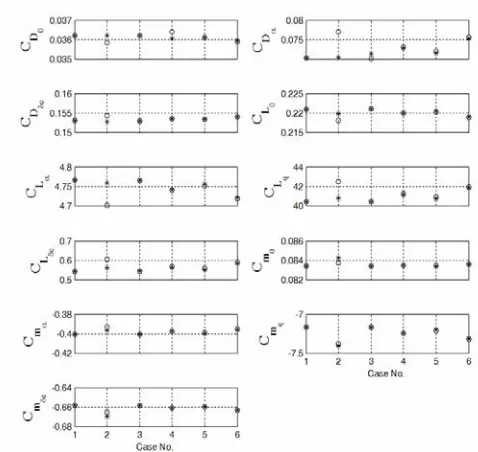
[image:5.612.74.289.179.322.2]Figure 5: Comparison of parameter values estimated through LM and GN optimization for FLT1, using various initial guess values of
parameters
The variation among the estimates obtained using LM and GN methods of updation of parameters is illustrated graphically in Fig. 5 for various cases of initial guess values. As seen in table 1, there was no appreciable difference observed among the derivatives obtained through LM and GN separately.
The estimated model obtained using FEM can be used to develop a mathematical model simulating longitudinal dynamics of HANSA-3 aircraft.
VI.CONCLUSION
The present task was to estimate and compare the numerical values of the estimated parameters obtained using EEM, OEM and FEM methods. To investigate the accuracy of the estimated model, Proof-of-Match exercise [12] was carried out.
It was observed that due to the turbulence in the atmosphere, an amount of process noise was introduced into the observation, along with certain measurement noise that was indispensible in the instrumentation of the aircraft.
EEM was first used for parameter estimation. Since EEM does not account for either measurement noise or process noise; the Proof-of-Match exercise clearly shows a large
deviation of the predicted variables through EEM from the measured variables.
Next, the Maximum Likelihood (ML) method (a variant of OEM) was used to estimate the values of the parameters. The system was assumed to be corrupted with measurement noise, which the method can duly handle. However in presence of turbulence OEM yields poor results in terms of convergence and estimate.
FEM yields satisfactory results even in presence of atmospheric turbulence, as it has capability to handle measurement and process noise. It was seen that by LM or by GN optimization, the present case did not prove to have much of advantages. However it is strongly believed that the LM method may be advantageous in presence of highly turbulent and highly nonlinear data in terms of convergence.
REFERENCES
[1] L. A. Zadeh, “From Circuit Theory to System Theory”, Proceeding of the IRE, Vol. 50, May 1962, pp. 856-965.
[2] P. G. Hamel, and R.V. Jategaonkar, “The Evolution of Flight Vehicle System Identification”, AGARD, DLR Germany, 8-10, May 1995. [3] K. W. Iliff, “Parameter Estimation for Flight Vehicle”, Journal of
Guidance, Control and Dynamics, Vol. 12, No. 5, 1989, pp609-622 [4] P. G. Hamel, “Aircraft Parameter Identification Methods and their
Applications Survey and Future Aspects”, AGARD, 13-104, Nov. 1979, Paper1.
[5] R. E. Maine, and K. W. Iliff, "Formulation and Implementation of a Practical Algorithm for Parameter Estimation with Process and Measurement Noise," Society for Industrial and Applied Mathematics Journal of Applied Mathematics, Vol. 41, Dec. 1981, pp. 558-579. [6] V. Klein, “Estimation of Aircraft Aerodynamic Parameter from Flight
Data”, Progress in Aerospace sciences, Vol. 26, 1989, pp1-77. [7] G. H. Bryan, Stability in Aviation, Mc Millan, London, 1911. [8] J. Roskam, “Methods for Estimating Stability and Control Derivatives
for conventional Subsonic Airplanes”, Roskam Aviation and Engineering Corporation, 1973.
[9] E. Seckel, and J. J. Morris, “The Stability Derivatives of the navion Aircraft Estimated by Various Methods and Derived from Flight test Data,” FAA-RD-71-6.
[10] E. Seckel, Stability and Control of Airplanes and Helicopters, Academic Press, New York, 1964.
[11] D. E. Hoak, and Ellision, D. E., USAF Stability and Control DATCOM; Air Force Flight Dynamics Laboratory, Wright Ptterson Airforce Base, Ohio, 1960, revised 1975.
[12] R. V. Jategaonkar, Flight Vehicle System Identification: A Time Domain Methodology, AIAA Progress in Aeronautics and Astronautics, Vol. 216, AIAA, Reston, VA, Aug 2006, Chaps. 4, 5 & 6.
[13] A. V. Balakrishnan, “Stochastic System Identification Techniques”, in stochastic Optimization and Control, edited by H.F. Karreman, John Wiley and Sons, London, 1968.
[14] R. Rangaranjan, and S. Vishwanathan, “Wind Tunnel Test Results on a 1/5 Scale HANSA Model,” NAL TR-01, Vol. 1, Dec. 1997. [15] R. V. Jategaonkar, and E. Plaetschke, "Estimation of Aircraft