A Comparative Study on Language Model Adaptation Techniques Using New Evaluation Metrics

A Comparative Study on Language Model Adaptation Techniques

Using New Evaluation Metrics

Hisami Suzuki

Jianfeng Gao

Microsoft Research Microsoft Research Asia

One Microsoft Way 49 Zhichun Road, Haidian District

Redmond WA 98052 USA Beijing 100080 China

[email protected] [email protected]

Abstract

This paper presents comparative experimen-tal results on four techniques of language model adaptation, including a maximum a posteriori (MAP) method and three dis-criminative training methods, the boosting algorithm, the average perceptron and the minimum sample risk method, on the task of Japanese Kana-Kanji conversion. We evalu-ate these techniques beyond simply using the character error rate (CER): the CER re-sults are interpreted using a metric of do-main similarity between background and adaptation domains, and are further evalu-ated by correlating them with a novel metric for measuring the side effects of adapted models. Using these metrics, we show that the discriminative methods are superior to a MAP-based method not only in terms of achieving larger CER reduction, but also of being more robust against the similarity of background and adaptation domains, and achieve larger CER reduction with fewer side effects.

1

Introduction

Language model (LM) adaptation attempts to ad-just the parameters of a LM so that it performs well on a particular (sub-)domain of data. Currently, most LMs are based on the Markov assumption that the prediction of a word depends only on the preceding n–1 words, but such n-gram statistics are known to be extremely susceptible to the charac-teristics of training samples. This is true even when the data sources are supposedly similar: for exam-ple, Rosenfeld (1996) showed that perplexity dou-bled when a LM trained on the Wall Street Journal (1987-1989) was tested on the AP newswire stories

of the same period. This observation, coupled with the fact that training data is available in large quan-tities only in selected domains, facilitates the need for LM adaptation.

There have been two formulations of the LM adaptation problem. One is the within-domain ad-aptation, in which adapted LMs are created for different topics in a single domain (e.g., Seymore and Rosenfeld, 1997; Clarkson and Robinson, 1997; Chen et al., 1998). In these studies, a domain is defined as a body of text originating from a sin-gle source, and the main goal of LM adaptation is to fine-tune the model parameters so as to improve the LM performance on a specific sub-domain (or topic) using the training data at hand.

The other formulation, which is the focus of the current study, is to adapt a LM to a novel domain, for which only a very small amount of training data is available. This is referred to as cross-domain adaptation. Following Bellegarda (2001), we call the domain used to train the original model the background domain, and the novel domain with a small amount of training data as the adapta-tion domain. Two major approaches to cross-domain adaptation have been investigated: maxi-mum a posteriori (MAP) estimation and discrimi-native training methods. In MAP estimation methods, adaptation data is used to adjust the pa-rameters of the background model so as to maxi-mize the likelihood of the adaptation data. Count merging and linear interpolation of models are the two MAP estimation methods investigated in speech recognition experiments (Iyer et al., 1997; Bacchiani and Roark, 2003), with count merging reported to slightly outperform linear interpolation.

2004) as well as adaptation (Bacchiani et al., 2004) scenarios.

In this paper, we present comparative experi-mental results on four language model adaptation techniques and evaluate them from various angles, attempting to elucidate the characteristics of these models. The four models we compare are a maxi-mum a posteriori (MAP) method and three dis-criminative training methods, namely the boosting algorithm (Collins, 2000), the average perceptron (Collins, 2002) and the minimum sample risk method (Gao et al., 2005). Our evaluation of these techniques is unique in that we go beyond simply comparing them in terms of character error rate (CER): we use a metric of distributional similarity to measure the distance between background and adaptation domains, and attempt to correlate it with the CER of each adaptation method. We also pro-pose a novel metric for measuring the side effects of adapted models using the notion of backward compatibility, which is very important from a soft-ware deployment perspective.

Our experiments are conducted in the setting of Japanese Kana-Kanji conversion, as we believe this task is excellently suited for evaluating LMs. We begin with the description of this task in the following section.

2

Language Modeling in the Task of IME

This paper studies language modeling in the con-text of Asian language (e.g., Chinese or Japanese) text input. The standard method for doing this is that the users first input the phonetic strings, which are then converted into the appropriate word string by software. The task of automatic conversion has been the subject of language modeling research in the context of Pinyin-to-Character conversion in Chinese (Gao et al., 2002a) and Kana-Kanji con-version in Japanese (Gao et al., 2002b). In this pa-per, we call the task IME (Input Method Editor), based on the name of the commonly used Win-dows-based application.

The performance of IME is typically measured by the character error rate (CER), which is the number of characters wrongly converted from the phonetic string divided by the number of charac-ters in the correct transcript. Current IME systems exhibit about 5-15% CER on real-world data in a wide variety of domains.

In many ways, IME is a similar task to speech recognition. The most obvious similarity is that IME can also be viewed as a Bayesian decision problem: let A be the input phonetic string (which corresponds to the acoustic signal in speech); the task of IME is to choose the most likely word string W* among those candidates that could have been converted from A:

) | ( ) ( max arg ) | ( max arg *

) ( )

(

W A P W P A

W P W

A W A

W∈GEN ∈GEN

=

= (1)

where GEN(A) denotes the candidate set given A. Unlike speech recognition, however, there is no acoustic ambiguity in IME, because the phonetic string is provided directly by users. Moreover, we can assume a unique mapping from W to A in IME, i.e., P(A|W) = 1. So the decision of Equation (1) depends solely on P(W), which makes IME ideal for testing language modeling techniques. Another advantage of using IME for language modeling research is that it is relatively easy to convert W to A, which facilitates the creation of training data for discriminative learning, as described later.

From the perspective of LM adaptation, IME faces the same problem speech recognition faces: the quality of the model depends heavily on the similarity of the training and test data. This poses a serious challenge to IME, as it is currently the most widely used method of inputting Chinese or Japa-nese characters, used by millions of users for in-putting text of any domain. LM adaptation in IME is therefore an imminent requirement for improv-ing user experience, not only as we build static domain-specific LMs, but also in making online user adaptation possible in the future.

3

Discriminative Algorithms for LM

Ad-aptation

This section describes three discriminative training methods we used in this study. For a detailed de-scription of each algorithm, readers are referred to Collins (2000) for the boosting algorithm, Collins (2002) for perceptron learning, and Gao et al. (2005) for the minimum sample risk method.

3.1 Definition

• Training data is a set of input-output pairs. In the task of IME, we have training samples {Ai, Wi

R }, for i = 1…M, where each Ai is an input phonetic string and each Wi

R

is the reference transcript of Ai. • We assume a set of D + 1 features fd(W), for d = 0…D. The features could be arbitrary functions that map W to real values. Using vector notation, we have f(W)∈ℜD+1, where f(W) = {f0(W), f1(W), …, fD(W)}. The feature f0(W) is called the base

model feature, and is defined as the log probability that the word trigram model assigns to W. The fea-tures fd(W) for d = 1…D are defined as the word n-gram counts (n = 1 and 2 in our experiments) in W. • The parameters of the model form a vector of D + 1 dimensions, one for each feature function, λ= {λ0, λ1, …, λD}. The likelihood score of a word string W can then be written as

) ( ) ,

(W W

Score λ =λf

∑

= D d

d df W

λ

0

)

( . (2)

Given a model λ and an input A, the decision rule of Equation (1) can then be rewritten as

). , ( max arg ) , (

* _{λ λ}

GEN W Score A W (A) W∈ = (3)

We can obtain the number of conversion errors in W by comparing it with the reference transcript WR using an error function Er(WR,W), which is an edit distance in our case. We call the sum of error counts over the training set the sample risk (SR). Discriminative training methods strive to optimize the parameters of a model by minimizing SR, as in Equation (4).

∑

i W A

W SR ... 1 * )) , ( , Er( min arg ) ( min

arg λ λ

λ

λ λ

(4)

However, (4) cannot be optimized directly by regu-lar gradient-based procedures as it is a piecewise constant function of λ and its gradient is undefined. The discriminative training methods described be-low differ in how they achieve the optimization: the boosting and perceptron algorithms approxi-mate SR by loss functions that are suitable for op-timization; the minimum sample risk method, on the other hand, uses a simple heuristic training pro-cedure to minimize SR directly without resorting to an approximated loss function.

3.2 The boosting algorithm

The boosting algorithm we used is based on Collins (2000). Instead of measuring the number of conversion errors directly, it uses a loss function

that measures the number of ranking errors, i.e., cases where an incorrect candidate W receives a higher score than the correct conversion WR. The margin of the pair (WR, W) with respect to the model λ is given by

) , ( ) , ( ) ,

(W W Score W λ Score W λ

M R = R − (5)

The loss function is then defined as

∑ ∑

= ∈

= M

i W_i A_i

i R i W W M I ...

1 ( )

)] , ( [ ) RLoss( GEN

λ (6)

where I[π] = 1 if π≤ 0, and 0 otherwise. Note that RLoss takes into account all candidates in GEN(A).

Since optimizing (6) is NP-complete, the boost-ing algorithm optimizes its upper bound:

∑ ∑

= ∈

− =

M

i W A

i R i i i W W M ...

1 ( )

)) , ( exp( ) ExpLoss( GEN

λ ₍₇₎

Figure 1 summarizes the boosting algorithm we used. After initialization, Step 2 and 3 are repeated N times; at each iteration, a feature is chosen and its weight is updated. We used the following up-date for the dth feature fd:

Z C Z C d d d _ε ε δ + + = log +_{_}

2

1 ₍₈₎

where Cd+ is a value increasing exponentially with

the sum of margins of (WR, W) pairs over the set where fd is seen in W

R

but not in W; Cd- is the value

related to the sum of margins over the set where fd is seen in W but not in WR. ε is a smoothing factor (whose value is optimized on held-out data) and Z is a normalization constant.

1 Set λ0 = 1 and λd = 0 for d=1…D

2 Select a feature fd which has largest estimated

im-pact on reducing ExpLoss of Equation (7)

3 _{Update λd by Equation (8),and return to Step 2}

Figure 1: The boosting algorithm

3.3 The perceptron algorithm

value for the dth parameter after the ith training sample has been processed in pass t over the train-ing data. The average parameters are defined as

). /( ) (

) (

1 1 ,

M T

T

t M

i i t d avg

d =

∑∑

= =

λ

λ (9)

3.4 The minimum sample risk method

The minimum sample risk (MSR, Gao et al., 2005) training algorithm is motivated by analogy with the feature selection procedure for the boosting algo-rithm (Freund et al., 1998). It is a greedy procedure for selecting a small subset of the features that have the largest contribution in reducing SR in a sequential manner. Conceptually, MSR operates like any multidimensional function optimization approach: a direction (i.e., feature) is selected and SR is minimized along that direction using a line search, i.e., adjusting the parameter of the selected feature while keeping all other parameters fixed. This is repeated until SR stops decreasing.

Regular numerical line search algorithms cannot be applied directly because, as described above, the value of a feature parameter versus SR is not smooth and there are many local minima. MSR thus adopts the method proposed by Och (2003). Let GEN(A) be the set of n-best candidate word strings that could be converted from A. By adjust-ing λd for a selected feature fd, we can find a set of intervals for λd within which a particular candidate word string is selected. We can compute Er(.) for the candidate and use it as the Er(.) value for the corresponding interval. As a result, we obtain an ordered sequence of Er(.) values and a correspond-ing sequence of λ intervals for each training sample. By summing Er(.) values over all training samples, we obtain a global sequence of SR and the corre-sponding global sequence of λd intervals. We can then find the optimal λd as well as its correspond-ing SR by traverscorrespond-ing the sequence.

Figure 3 summarizes the MSR algorithm. See Gao et al. (2005) for a complete description of the

MSR implementation and the empirical justifica-tion for its performance.

4

Experimental Results

4.1 Data

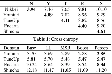
The data used in our experiments come from five distinct sources of text. A 36-million-word Nikkei newspaper corpus was used as the background domain. We used four adaptation domains: Yomi-uri (newspaper corpus), TuneUp (balanced corpus containing newspaper and other sources of text), Encarta (encyclopedia) and Shincho (collection of novels). The characteristics of these domains are measured using the information theoretic notion of cross entropy, which is described in the next sub-section.

For the experiment of LM adaptation, we used the training data consisting of 8,000 sentences and test data of 5,000 sentences from each adaptation domain. Another 5,000-sentence subset was used as held-out data for each domain, which was used to determine the values of tunable parameters. All the corpora used in our experiments are pre-segmented into words using a baseline lexicon consisting of 167,107 entries.

4.2 Computation of domain characteristics

Yuan et al. (2005) introduces two notions of do-main characteristics: a within-dodo-main notion of diversity, and a cross-domain concept of similarity. Diversity is measured by the entropy of the corpus and indicates the inherent variability within the domain. Similarity, on the other hand, is intended to capture the difficulty of a given adaptation task, and is measured by the cross entropy.

For the computation of these metrics, we ex-tracted 1 million words from the training data of each domain respectively, and created a lexicon consisting of the words in our baseline lexicon plus all words in the corpora used for this experiment (resulting in 216,565 entries) to avoid the effect of out-of-vocabulary items. Given two domains A and

1 Set λ0 = 1 and λd = 0 for d=1…D

2 For t = 1…T (T = the total number of iterations)

3 For each training sample (Ai, WiR), i = 1…M

4 Choose the best candidate Wi from GEN(Ai)

according to Equation (3)

5 For each λd (η = size of learning step)

6 λd = λd + η(fd(WiR) – fd(Wi))

Figure 2: The perceptron algorithm

1 Set λ0 = 1 and λd = 0 for d=1…D

2 Rank all features by its expected impact on reduc-ing SR and select the top N features

3 For each n = 1…N

4 Update the parameter of f using line search

B, we then trained a word trigram model for each domain B, and used the resulting model in comput-ing the cross entropy of domain A. For simplicity, we denote this as H(A,B).

Table 1 summarizes our corpora along this di-mension. Note that the cross entropy is not sym-metric, i.e., H(A,B) is not necessarily the same as H(B,A), so we only present the average cross en-tropy in Table 1. We can observe that Yomiuri and TuneUp are much more similar to the background Nikkei corpus than Encarta and Shincho.

H(A,A) along the diagonal of Table 1 (in bold-face) is the entropy of the corpus, indicating the corpus diversity. This quantity indeed reflects the in-domain variability of text: newspaper and ency-clopedia articles are highly edited text, following style guidelines and often with repetitious content. In contrast, Shincho is a collection of novels, on which no style or content restriction is imposed. We use these metrics in the interpretation of CER results in Section 5.

4.3 Results of LM adaptation

The discriminative training procedure was carried out as follows: for each input phonetic string A in the adaptation training set, we produced a word lattice using the baseline trigram models described in Gao et al. (2002b). We kept the top 20 hypothe-ses from this lattice as the candidate conversion set

GEN(A). The lowest CER hypothesis in the lattice

rather than the reference transcript was used as WR. We used unigram and bigram features that oc-curred more than once in the training set.

We compared the performance of discriminative methods against a MAP estimation method as the baseline, in this case the linear interpolation

method. Specifically, we created a word trigram model using the adaptation data for each domain, which was then linearly interpolated at the word level with the baseline model. The probability ac-cording to the combined model is given by

) | ( ) 1 ( ) | ( ) |

(w h P w h P w h

p i

A i

B

i =λ + −λ ,

where PB is the probability of the background model, PA the probability of the adaptation model, and the history h corresponds to two preceding words. λ was tuned using the held-out data.

In evaluating both MAP estimation and dis-criminative models, we used an N-best rescoring approach. That is, we created N best hypotheses using the baseline trigram model (N=100 in our experiments) for each sentence in the test data, and used adapted models to rescore the N-best list. The oracle CERs (i.e., the minimal possible CER given the available hypotheses) ranged from 1.45% to 5.09% depending on the adaptation domain.

The results of the experiments are shown in Ta-ble 2. We can make some observations from the table. First, all discriminative methods signifi-cantly outperform the linear interpolation (statisti-cally significant according to the t-test at p < 0.01). In contrast, the differences among three discrimi-native methods are very subtle and most of them are not statistically significant. Secondly, the CER results correlate well with the metric of domain similarity in Table 1 (r=0.94 using the Pearson product moment correlation coefficient). This is consistent with our intuition that the closer the ad-aptation domain is to the background domain, the easier the adaptation task.

Regarding the similarity of the adaptation do-main to the background, we also observe that the CER reduction of the linear interpolation model is particularly limited when the adaptation domain is similar to the background domain: the CER reduc-tion of the linear interpolareduc-tion model for Yomiuri and TuneUp over the baseline is 0% and 1.89% respectively, in contrast to ~22% and ~5.8% im-provements achieved by the discriminative models. The discriminative methods are therefore more robust against the similarity of the adaptation and background data than the linear interpolation.

Our results differ from Bacchiani et al. (2004) in that in our system, the perceptron algorithm alone achieved better results than MAP estimation. However, the difference may only be apparent, given different experimental settings for the two

N Y T E S

Nikkei 3.94 7.46 7.65 9.81 10.10

Yomiuri 4.09 7.82 8.96 9.29

TuneUp 4.41 8.82 8.56

Encarta 4.40 9.20

Shincho 4.61

Table 1: Cross entropy

Domain Base LI MSR Boost Percep

Yomiuri 3.70 3.69 2.89 2.88 2.85

TuneUp 5.81 5.70 5.48 5.47 5.47

Encarta 10.24 8.64 8.39 8.54 8.34

Shincho 12.18 11.47 11.05 11.09 11.20

studies. We used the N-best reranking approach with the same N-best list for both MAP estimation and discriminative training, while in Bacchiani et al. (2004), two different lattices were used: the per-ceptron model was applied to rerank the lattice created by the background model, while the MAP adaptation model was used to produce the lattice itself. The fact that the combination of these mod-els (i.e., first use the MAP estimation to create hy-potheses and then use the perceptron algorithm to rerank them) produced the best results indicates that given a candidate lattice, the perceptron algo-rithm is effective in candidate reranking, thus mak-ing our results compatible with theirs.

5

Discussion

The results in Section 4 demonstrate that discrimi-native training methods for adaptation are overall superior to MAP adaptation methods. In this sec-tion, we show additional advantages of discrimina-tive methods beyond simple CER improvements.

5.1 Using metrics for side effects

In the actual deployment of LM adaptation, one issue that bears particular importance is the num-ber of side effects that are introduced by an adapted model. For example, consider an adapted model which achieves 10% CER improvements over the baseline. Such a model can be obtained by improving 10%, or by improving 20% and by in-troducing 10% of new errors. Clearly, the former model is preferred, particularly if the models be-fore and after adaptation are both to be exposed to users. This concept is more widely acknowledged within the software industry as backward compati-bility – a requirement that an updated version of software supports all features of its earlier versions. In IME, it means that all phonetic strings that can be converted correctly by the earlier versions of the system should also be converted correctly by the new system as much as possible. Users are typi-cally more intolerant to seeing errors on the strings that used to be converted correctly than seeing er-rors that also existed in the previous version. Therefore, it is crucial that when we adapt to a new domain, we do so by introducing the smallest number of side effects, particularly in the case of an incremental adaptation to the domain of a par-ticular user, i.e., to building a model with incre-mental learning capabilities.

5.2 Error ratio

In order to measure side effects, we introduce the notion of error ratio (ER), which is defined as

| |

| |

B A

E E ER= ,

where |EA| is the number of errors found only in the new (adaptation) model, and |EB| the number of errors corrected by the new model. Intuitively, this quantity captures the cost of improvement in the adaptation model, corresponding to the number of newly introduced errors per each improvement. The smaller the ratio is, the better the model is at the same CER: ER=0 if the adapted model intro-duces no new errors, ER<1 if the adapted model makes CER improvements, ER=1 if the CER im-provement is zero (i.e., the adapted model makes as many new mistakes as it corrects old mistakes), and ER>1 when the adapted model has worse CER performance than the baseline model.

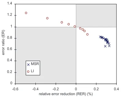
Given the notion of CER and ER, a model can be plotted on a graph as in Figure 4: the relative error reduction (RER, i.e., the CER difference be-tween the background and adapted models) is plot-ted along the x-axis, and ER along the y-axis. Figure 4 plots the models obtained after various numbers of iterations for MSR training and at vari-ous interpolation weights for linear interpolation for the TuneUp domain. The points in the upper-left quadrant, ER>1 and RER<0, are the models that performed worse than the baseline model (some of the interpolated models fall into this cate-gory); the shaded areas (upper-right and lower-left quadrants) are by definition empty. The lower-right quadrant is the area of interest to us, as they

0 0.2 0.4 0.6 0.8 1 1.2 1.4

-0.6 -0.4 -0.2 0 0.2 0.4

MSR LI

represent the models that led to CER improve-ments; we will focus only on this area now in Figure 5.

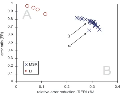
In this figure, a model is considered to have fewer side effects when the ER is smaller at the same RER (i.e., smaller value of y for a fixed value of x), or when the RER is larger at the same ER (i.e., larger value of x at the fixed y). That is, the closer a model is plotted to the corner B of the graph, the better the model is; the closer it is to the corner A, the worse the model is.

5.3 Model comparison using RER/ER

From Figure 5, we can clearly see that MSR mod-els have better RER/ER-performance than linear interpolation models, as they are plotted closer to the corner B. Figure 6 displays the same plot for all four domains: the same trend is clear from all

graphs. We can therefore conclude that a discrimi-native method (in this case MSR) is superior to linear interpolation not only in terms of CER re-duction, but also of having fewer side effects. This desirable result is attributed to the nature of dis-criminative training, which works specifically to adjust feature weights so as to minimize error.

Figure 7: RER/ER plot for MSR, boosting and percep-tron models (X-axis is normalized to represent relative

error rate reduction)

Figure 7 compares the three discriminative models with respect to RER/ER by plotting the best models (i.e., models used to produce the re-sults in Table 1) for each algorithm. We can see that even though the boosting and perceptron algo-rithms have the same CER for Yomiuri and TuneUp from Table 2, the perceptron is better in terms of ER; this may be due to the use of expo-nential loss function in the boosting algorithm which is less robust against noisy data (Hastie et al., 2001). We also observe that Yomiuri and Encarta do better in terms of side effects than TuneUp and Shincho for all algorithms, which can be explained by corpus diversity, as the former set is less stylis-tically diverse and thus more consistent within the domain.

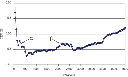
5.4 Overfitting and side effects

The RER/ER graph also casts the problem of over-fitting in an interesting perspective. Figure 8 is de-rived from running MSR on the TuneUp test corpus, which depicts a typical case of overfitting: the CER drops in the beginning, but after a certain number of iterations, it goes up again. The models indicated by α and β in the graph are of the same CER, and as such, these models are equivalent. When plotted on the RER/ER graph in Figure 5,

0 0.1 0.2 0.3 0.4 0.5 0.6 0.7 0.8 0.9 1

0 0.1 0.2 0.3 0.4 MSR

LI

A

B

Figure 5: RER/ER plot for the models with ER<1 and RER>0 for TuneUp domain. See Figure 8 for the

de-scription of α and β

0 0.1 0.2 0.3 0.4 0.5 0.6 0.7 0.8 0.9 1

0 0.2 0.4 0.6 0.8 1 1.2 1.4 1.6 1.8 2 0 0.1 0.2 0.3 0.4 0.5 0.6 0.7 0.8 0.9 1

0 0.05 0.1 0.15 0.2 0.25 0.3 0.35

0 0.1 0.2 0.3 0.4 0.5 0.6 0.7 0.8 0.9 1

0 0.2 0.4 0.6 0.8 1 1.2 0

0.1 0.2 0.3 0.4 0.5 0.6 0.7 0.8 0.9 1

0 0.1 0.2 0.3 0.4 0.5 0.6 0.7 0.8 0.9

Yomiuri TuneUp

Encarta Shincho

Figure 6: RER/ER plot for all four domains x-axes: RER (%); y-axes: ER

however, it is clear that the overfit model β has the worse ER than the non-overfit counterpart α. In other words, models α and β have the same CER, but they are not equivalent: model β is not only worse in light of containing more features, but also in terms of causing more side effects.

6

Conclusion and Future Work

We have presented a comparison of three discrimi-native learning approaches with a MAP estimation method in the task of LM adaptation for IME. We have shown that all discriminative models are sig-nificantly better than the linear interpolation method, in that they achieve larger CER reduction with fewer side effects across different domains.

One direction of future research is to apply this technique to an incremental learning scenario, i.e., to incrementally build models using incoming data for adaptation, taking all previously available data as background corpus. The new metric for back-ward compatibility we proposed in the paper will play a particularly important role in such a scenario.

Acknowledgements

We would like to thank Kevin Duh, Gary Kacmar-cik, Eric Ringger, Yoshiharu Sato and Wei Yuan for their help at various stages of this research.

References

Bacchiani, M. and B. Roark. 2003. Unsupervised Lan-guage Model Adaptation. Proceedings of ICASSP, pp.224-227.

Bacchiani, M., B. Roark and M. Saraclar. 2004. Lan-guage Model Adaptation with MAP Estimation and the Perceptron Algorithm. Proceedings of

HLT-NAACL, pp.21-24.

Bellegarda, J.R. 2001. An Overview of Statistical Lan-guage Model Adaptation. ITRW on Adaptation

Meth-ods for Speech Recognition, pp. 165-174.

Chen, S.F., K. Seymore and R. Rosenfeld. 1998. Topic Adaptation for Language Modeling Using Unnormal-ized Exponential Models. Proceedings of ICASSP.

Clarkson, P.R., and A.J. Robinson. 1997. Language Model Adaptation Using Mixtures and an Exponen-tially Decaying Cache. Proceedings of ICASSP. Collins, M. 2000. Discriminative Reranking for Natural

Language Parsing. ICML 2000.

Collins, M. 2002. Discriminative Training Methods for Hidden Markov Models: Theory and Experiments with Perceptron Algorithm. Proceedings of EMNLP, pp.1-8.

Freund, Y., R. Iyer, R.E. Shapire and Y. Singer. 1998 An Efficient Boosting Algorithm for Combining Pref-erences. ICML'98.

Gao, J., J. Goodman, M. Li and K.-F. Lee. 2002a. To-ward a unified approach to statistical language model-ing for Chinese. ACM Transactions on Asian

Language Information Processing, 1-1: 3-33.

Gao, J, H. Suzuki and Y. Wen. 2002b. Using Headword Dependency and Predictive Clustering for Language Modeling. Proceedings of EMNLP: 248-256.

Gao, J., H. Yu, P. Xu and W. Yuan. 2005. Minimum Sample Risk Methods for Language Modeling.

Pro-ceedings of EMNLP 2005.

Hastie, T., R. Tibshirani and J. Friedman. 2001. The

Elements of Statistical Learning. Springer-Verlag,

New York.

Iyer, R., M. Ostendorf and H. Gish. 1997. Using Out-of-Domain Data to Improve In-Out-of-Domain Language Models.

IEEE Signal Processing Letters, 4-8: 221-223.

Mitchell, Tom M. 1997. Machine learning. The McGraw-Hill Companies, Inc.

Och, F. J. 2003. Minimum Error Rate Training in Statis-tical Machine Translation. Proceedings of ACL: 160-167.

Roark, B., M. Saraclar and M. Collins. 2004. Corrective Language Modeling for Large Vocabulary ASR with the Perceptron Algorithm. Proceedings of ICASSP: 749-752.

Rosenfeld, R. 1996. A Maximum Entropy Approach to Adaptive Statistical Language Modeling. Computer,

Speech and Language, 10: 187-228.

Seymore, K. and R. Rosenfeld. 1997. Using Story Top-ics For Language Model Adaptation. Proceedings of

Eurospeech '97.

Yuan, W., J. Gao and H. Suzuki. 2005. An Empirical Study on Language Model Adaptation Using a Metric of Domain Similarity. Proceedings of IJCNLP 05.

5.45 5.5 5.55 5.6 5.65

0 500 1000 1500 2000 2500 3000 3500 4000 4500 5000