HGSGNLP at IEST 2018: An Ensemble of Machine Learning and Deep Neural Architectures for Implicit Emotion Classification in Tweets

Proceedings of the 9th Workshop on Computational Approaches to Subjectivity, Sentiment and Social Media Analysis, pages 205–210 205

HGSGNLP at IEST 2018: An Ensemble of Machine Learning and Deep

Neural Architectures for Implicit Emotion Classification in Tweets

WenTing Wang1, Man Lan2

1_{Alibaba Group, WenYi West Road #969, Hangzhou City} 2_{Department of Computer Science and Technology,}

East China Normal University, Shanghai, P.R.China

[email protected], [email protected]

Abstract

This paper describes our system designed for the WASSA-2018 Implicit Emotion Shared Task (IEST). The task is to predict the emo-tion category expressed in a tweet by remov-ing the termsangry,afraid,happy,sad, sur-prised,disgustedand their synonyms. Our fi-nal submission is an ensemble of one super-vised learning model and three deep neural network based models, where each model ap-proaches the problem from essentially differ-ent directions. Our system achieves the macro F1 score of 65.8%, which is a 5.9% perfor-mance improvement over the baseline and is ranked 12 out of 30 participating teams.

1 Introduction

In Natural Language Processing, emotion recog-nition is concerning of associating words, phrases or documents with predefined emotion categories, such as Anger, Anticipation and Sadness (Ekman, 1999;Plutchik,2001). Most of previous research works on emotion recognition (Wang et al.,2012; Bestgen and Vincze,2012;Suttles and Ide,2013; Recchia and Louwerse,2015;Hollis et al.,2017) presumes emotion words or their representations are accessible. Such models might fail to learn as-sociations for more subtle descriptions and there-fore fail to predict the emotion when overt emotion words are not available.

The WASSA-2018 Implicit Emotion Shared Task (IEST) (Klinger et al.,2018) aims to predict the emotion category of a given tweet when the ex-plicit emotion word, ortrigger words, is removed. The emotion category can be one of six classes: Anger,Disgust, Fear,Joy, SadnessandSurprise. For examples:

1. “It’s [#TARGETWORD#] when you feel like you are invisible to others.”

2. “We are so [#TARGETWORD#] that people must think we are on good drugs or just really good actors.”

In the above 2 examples, with the help of com-mon sense or world knowledge, implicit emotion still can be inferred from context as Sadnessand Joy. The [#TARGETWORD#] tokens in the ex-amples indicate the position of the removed word in the given tweet.

Our submitted system is an ensemble of four broad sets of approaches combined using a weighted average of the separate predictions. One approach uses traditional lexicon-based method to train a logistic regression classifier, while the re-maining three approaches rely on representing the input tweet as a word vector and using neural net-work based architectures to give the emotion cate-gory for the tweet.

The rest of the paper is structured as follows. Section 2 describes the features used in our sys-tem. Section 3 explains the various approaches used by our ensemble model and the way we com-bined the predictions. Section 4 states the ex-periment results and discusses the implications of those results. We conclude our work in Section5.

2 Features

2.1 Word

The current word and its lowercase format are used as features. To provide additional context information, word n-grams and character n-grams are also used.

2.2 Word Embeddings

Word embeddings are trained from large unlabeled raw tweets to be used as input to neural network model as well as for generating word clusters.

Arguments Value

–oaa 6

–loss function logistic

–passes 10

–ngram b3

–skips b2

–affix +3b,-1b

-l 0.3

Table 1: Vowpal Wabbit command line arguments used to train the model. The namespacebdenotes lowercase word feature.

contain emotion word found in the NRC Emotion Lexicon. In addition, the word to the left and right of the emotion word are constrained to those words found in the training data. This constraint is used to remove tweets containing generic context such as “happy birthday”. After filtering, the final tweet collection contains 11 million tweets.

From this tweet collection, word embeddings are generated following the steps described in Toh and Su (2016). Besides using the previous two approaches (Gensim and GloVe tool), the fastText tool (Bojanowski et al.,2017)1is also used to gen-erate word embeddings.

2.3 Word Cluster

K-means clusters are generated from the word em-beddings using the K-means implementation of Apache Spark MLlib. From the K-means clus-ters, word cluster features are generated. For each word, the cluster id that the word belongs to is used as a feature.

3 Approaches

This section describes the four approaches used to generate the emotion predictions.

3.1 Approach 1: Lexicon Model

The Vowpal Wabbit tool2 is used to train a mul-ticlass classifier using the one-against-all setting (--oaa).

The features used to train the classifier include the words in the tweet (both original and lowercase format) and word clusters where 5 different word clusters are used.

Table 1 shows the command line arguments used to train the Vowpal Wabbit model.

1

https://fasttext.cc/

2_{https://github.com/JohnLangford/vowpal wabbit/wiki}

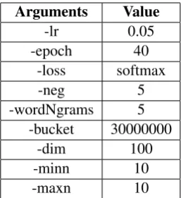
Arguments Value

-lr 0.05

-epoch 40

-loss softmax

-neg 5

-wordNgrams 5 -bucket 30000000

-dim 100

-minn 10

-maxn 10

Table 2: fastText command line arguments used to train the model.

3.2 Approach 2: fastText Model

The fastText tool is used to train a text classi-fier using thesupervisedsubcommand (Joulin et al.,2017).

The lowercase words in the tweet are used to train the classifier.

Table 2 shows the command line arguments used to train the fastText model.

3.3 Approach 3: Convolutional Neural Network Model

Convolutional Neural Network (CNN) has been shown to work well for sentence-level classifica-tion tasks (Kim,2014). Here we detail the archi-tecture of our network.

Input and Embedding Layer: Each tweet is preprocessed by (1) normalizing emoji to text3; (2) normalizing hyper links and @mentions to someurl and someuser; and (3) splitting hashtag chunks into separate words4. Then the tweet is converted into a concatenated vector and padded to an equal length (or truncated if the tweet is longer than the pre-defined length). The input vector is fed to the embedding layer (i.e. pre-trained glove.twitter.27B vectors), which converts each word into a distributional vector.

CNN Layer: The concatenated vector represen-tation of the tweet is then fed to CNN. The number of hidden units is set to be 256. We applytanhas activation and dropout with a rate of 0.2.

Output Layer: The output of CNN is flattened and then passed to a fully connected layer. Finally, a softmax layer was added on top of the fully con-nected layer. The network is trained by

minimiz-3

https://pypi.org/project/emoji

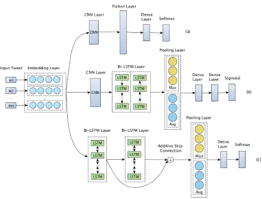
Figure 1: The architectures of our three neural models. (a) is the neural model for Approach 3. (b) is the neural model for Approach 4. (c) is the neural model for Approach 5.

ing the categorical cross-entropy error with RM-SProp for parameter optimization.

Figure1(a) shows the model architecture of the CNN model.

3.4 Approach 4: Sequence Modeling using CNN and LSTM

Long-short Term Memory (LSTM) (Hochreiter and Schmidhuber, 1997) architecture is an ad-vanced version of RNN and has been success-ful in the NLP domain on various tasks (Graves and Schmidhuber,2005;Graves and Jaitly,2014). Combining CNN and LSTM has also been found to be quite successful in (Zhou et al.,2015;Goel et al.,2017). In this approach, we attempt to use CNN to extract regional features and then use Bi-LSTM to capture compositional semantics from both forward and backward directions of word se-quence.

Since the input, embedding, CNN layers are the same as Approach 2, we only detail the architec-tures of the following different layers.

Bi-LSTM with Pooling Layer: We use bi-directional LSTMs followed by some pooling layer to model the output from CNN layer. The

number of hidden units is set to be 300. We ap-ply relu as activation and dropout with a rate of 0.2. The outcomes from max pooling and average pooling are concatenated.

Output Layer: The concatenated output of Bi-LSTM with Pooling layer is then passed to a fully connected layer. Finally, a sigmoid layer was added on top of the fully connected layer. The network is trained by minimizing the categorical cross-entropy error with Adam for parameter opti-mization.

Figure1(b) shows the model architecture of the sequence model.

3.5 Approach 5: Residual LSTM Model

Residual LSTM (Kim et al.,2017) adds an addi-tional spatial shortcut path from lower layers to better deal with vanishing gradients. It provides efficient training of deep networks with multiple LSTM layers and has been successfully applied to speech recognition and NER tasks (Tran et al., 2017). The formulation is as follows:

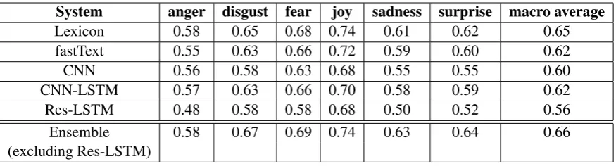
System anger disgust fear joy sadness surprise macro average

Lexicon 0.58 0.65 0.68 0.74 0.61 0.62 0.65

fastText 0.55 0.63 0.66 0.72 0.59 0.60 0.62

CNN 0.56 0.58 0.63 0.68 0.55 0.55 0.60

CNN-LSTM 0.57 0.63 0.66 0.70 0.58 0.59 0.62

Res-LSTM 0.48 0.58 0.58 0.68 0.50 0.52 0.56

Ensemble 0.58 0.67 0.69 0.74 0.63 0.64 0.66

(excluding Res-LSTM)

Table 3: Performance comparison between individual models and ensemble model on trial data. Our final ensemble model includes lexicon, fastText, CNN and CNN-LSTM models.

f_tl=σ(W_xfl xl_t+W_hfl hl_t−1+wcfl clt−1+blf) (2)

cl_t=f_tl·c_tl−1+ilt·tanh(Wxcl xlt+Whcl hlt−1+blc) (3)

ol_t=σ(W_xol xl_t+W_hol h_tl−1+wlcoclt+blo) (4)

r_tl=tanh(cl_t) (5)

ml_t=W_ol·rl_t (6)

hl_t=ol_t·(ml_t+xl_t) (7)

Where l represents layer index and il

t, ftl and

ol_t are input, forget and output gates respectively.

xl_t is an input from(l−1)th layer,hl_t−1 is a out-put layer at timet−1andcl_t−1 is an internal cell state att−1. And a short cut from a prior output layerhl_t−1 is added to a projection output ml_tvia

W_hlxl_t=W_hlhl_t−1

Figure1(c) shows the model architecture of our residual LSTM model. Two Bi-LSTM layers are included and the number of hidden units is set to be 512. We apply relu as activation and dropout with a rate of 0.2. The network is then trained by minimizing the categorical cross-entropy error with Adam for parameter optimization.

3.6 Ensemble Model

To combine the predictions of the five models mentioned above, we compute the weighted aver-age of the category probabilities of the four mod-els. The trial data is used to select the optimal weight of each model. The selected emotion cate-gory is the catecate-gory that has the highest weighted average.

4 Experiments and Results

4.1 Dataset and Evaluation Metric

The task organizers provide a training dataset (i.e. 153k instances) and a small blind trial dataset (i.e. 9.6k instances) for system building. Then a period of 1 week is given for submitting the predictions on a blind test dataset (i.e. 29k instances).

Macro-averaged F1 score is chosen to be the of-ficial evaluation metric.

4.2 Results on Trial Data and Analysis

The optimal setting for each model is decided using cross validation on training dataset. Then the weighted average is computed from individual predictions to generate the predictions for the final ensemble model using trial dataset as described in Section3.6. Table3shows the trial results for all individual models and ensemble model.

We observe that the Lexicon approach achieves the best score among all approaches. Among the four deep neural models, CNN+LSTM and fast-Text achieve better score of 62% compared to CNN and Residual-LSTM, which demonstrates that both the combination of long sequence and regional features and the word n-grams capture ef-fective information. Since the residual LSTM net-work does not perform as expected, we did not in-clude it into our final ensemble model.

We also observe that the ensemble model achieves the best performance compared with each individual model and offers equal or better per-formance across all the emotions, which indi-cates that the four approaches do complement each other quite well.

4.3 Official Results on Test Data

Label TP FP FN Precision Recall F1 anger 2814 1922 1980 0.594 0.587 0.591 disgust 3168 1537 1626 0.673 0.661 0.667

fear 3292 1455 1499 0.693 0.687 0.690

joy 3949 1342 1297 0.746 0.753 0.750

sad 2547 1290 1793 0.664 0.587 0.623

surprise 3212 2229 1580 0.590 0.670 0.628 Micro Average 18982 9775 9775 0.660 0.660 0.660 Macro Average 0.660 0.657 0.658

Table 4: Official results for our submission.

System anger disgust fear joy sadness surprise macro average Our Submission 0.59 0.67 0.69 0.75 0.62 0.63 0.658 (12)

Baseline 0.52 0.62 0.63 0.70 0.56 0.57 0.599

Amobee 0.64 0.72 0.75 0.82 0.69 0.68 0.714 (1)

IIIDYT 0.64 0.71 0.75 0.80 0.69 0.68 0.710 (2)

NTUA-SLP 0.63 0.71 0.74 0.79 0.69 0.67 0.703 (3)

Table 5: Performance comparison between our system, official baseline system and top-ranked systems on IEST shared task. The number in parentheses are the official rankings.

model gives the best performance for Joy, fol-lowed byFearandDisgust.

We also compare the results achieved by our submitted ensemble system, official baseline sys-tem and top-ranked syssys-tems in Table5. Our en-semble model achieves average f1-macro score of 65.8%, which beats the baseline model by 5.9%. However, the top-ranked systems all incorporate models trained in previous emotion related tasks (e.g. SemEval 2018: Affective in Tweets) as addi-tional features. This probably is the reason for our performance gap.

5 Conclusion and Future Work

In this paper, we propose a hybrid framework to predict the emotion category in tweets when no explicit emotion words are presented. The pro-posed approach combines lexicon based logistic regression classifier, fastText, Convolutional Neu-ral Networks and Sequence Modeling using CNN and LSTM, allowing us to explore the different di-rections each methodology can take. Our system HGSGNLP, submitted to the IEST 2018 Shared Task, beats the baseline system by 5.9% on the test set.

Compared to the best systems, there is still room for improvement. In the future, we would like to experiment with some other filters

provided in AffectiveTweets package (Mo-hammad and Bravo-Marquez, 2017) such as TweetToSentiStrengthFeatureVector. We would also experiment with incorporating lexicon features to existing neural networks.

References

Yves Bestgen and Nadja Vincze. 2012. Checking and bootstrapping lexical norms by means of word similarity indexes. Behavior research methods, 44(4):998–1006.

Piotr Bojanowski, Edouard Grave, Armand Joulin, and Tomas Mikolov. 2017. Enriching word vectors with subword information. Transactions of the Associa-tion for ComputaAssocia-tional Linguistics, 5:135–146.

Paul Ekman. 1999. Basic emotions. Handbook of cog-nition and emotion, pages 45–60.

Pranav Goel, Devang Kulshreshtha, Prayas Jain, and Kaushal Kumar Shukla. 2017. Prayas at emoint 2017: An ensemble of deep neural architectures for emotion intensity prediction in tweets. In Pro-ceedings of the 8th Workshop on Computational Ap-proaches to Subjectivity, Sentiment and Social Me-dia Analysis, pages 58–65.

Alex Graves and J¨urgen Schmidhuber. 2005. Frame-wise phoneme classification with bidirectional lstm and other neural network architectures. Neural Net-works, 18(5-6):602–610.

Sepp Hochreiter and J¨urgen Schmidhuber. 1997. Long short-term memory. Neural computation, 9(8):1735–1780.

Geoff Hollis, Chris Westbury, and Lianne Lefsrud. 2017. Extrapolating human judgments from skip-gram vector representations of word meaning. The Quarterly Journal of Experimental Psychology, 70(8):1603–1619.

Armand Joulin, Edouard Grave, Piotr Bojanowski, and Tomas Mikolov. 2017. Bag of tricks for efficient text classification. InProceedings of the 15th Con-ference of the European Chapter of the Association for Computational Linguistics: Volume 2, Short Pa-pers, pages 427–431. Association for Computational Linguistics.

Jaeyoung Kim, Mostafa El-Khamy, and Jungwon Lee. 2017. Residual lstm: Design of a deep recurrent ar-chitecture for distant speech recognition. In INTER-SPEECH.

Yoon Kim. 2014. Convolutional neural networks for sentence classification. InProceedings of the 2014 Conference on Empirical Methods in Natural Lan-guage Processing (EMNLP), pages 1746–1751. As-sociation for Computational Linguistics.

Roman Klinger, Orph´ee de Clercq, Saif M. Moham-mad, and Alexandra Balahur. 2018. Iest: Wassa-2018 implicit emotions shared task. InProceedings of the 9th Workshop on Computational Approaches to Subjectivity, Sentiment and Social Media Anal-ysis, Brussels, Belgium. Association for Computa-tional Linguistics.

Saif Mohammad and Felipe Bravo-Marquez. 2017. Wassa-2017 shared task on emotion intensity. In Proceedings of the 8th Workshop on Computational Approaches to Subjectivity, Sentiment and Social Media Analysis, pages 34–49. Association for Com-putational Linguistics.

Robert Plutchik. 2001. The nature of emotions: Hu-man emotions have deep evolutionary roots, a fact that may explain their complexity and provide tools for clinical practice. American scientist, 89(4):344– 350.

Gabriel Recchia and Max M Louwerse. 2015. Repro-ducing affective norms with lexical co-occurrence statistics: Predicting valence, arousal, and domi-nance. The Quarterly Journal of Experimental Psy-chology, 68(8):1584–1598.

Jared Suttles and Nancy Ide. 2013. Distant supervision for emotion classification with discrete binary val-ues. InInternational Conference on Intelligent Text Processing and Computational Linguistics, pages 121–136. Springer.

Toh, Zhiqiang and Su, Jian. 2016. NLANGP at SemEval-2016 Task 5: Improving Aspect Based Sentiment Analysis using Neural Network Fea-tures. In Proceedings of the 10th International Workshop on Semantic Evaluation (SemEval-2016), pages 282–288. Association for Computational Lin-guistics.

Quan Tran, Andrew MacKinlay, and Antonio Ji-meno Yepes. 2017. Named entity recognition with stack residual lstm and trainable bias decoding. In Proceedings of the Eighth International Joint Con-ference on Natural Language Processing (Volume 1: Long Papers), pages 566–575. Asian Federation of Natural Language Processing.

Wenbo Wang, Lu Chen, Krishnaprasad Thirunarayan, and Amit P Sheth. 2012. Harnessing twitter” big data” for automatic emotion identification. In Privacy, Security, Risk and Trust (PASSAT), 2012 International Conference on and 2012 Interna-tional Confernece on Social Computing (Social-Com), pages 587–592. IEEE.