Adaptive Convolution for Text Classification

2475

Adaptive Convolution for Text Classification

Byung-Ju Choi Jun-Hyung Park SangKeun Lee Department of Computer Science and Engineering

Korea University, Korea

{bj1123, irish07, yalphy}@korea.ac.kr

Abstract

In this paper, we present an adaptive convolution for text classification to give stronger flexibility to convolutional neural networks (CNNs). Unlike traditional convolutions that use the same set of filters regardless of different inputs, the adaptive convolution employs adaptively generated convolutional filters that are conditioned on inputs. We achieve this by attaching filter-generating networks, which are carefully designed to generate input-specific filters, to convolution blocks in existing CNNs. We show the efficacy of our approach in existing CNNs based on our performance evaluation. Our evaluation indicates that adaptive convolutions improve all the baselines, without any exception, as much as up to 2.6 percentage point in seven benchmark text classification datasets.

1 Introduction

Text classification assigns topics to texts by understanding the semantics of the texts. It is one of the fundamental tasks in natural language processing (NLP) which has a broad range of applications, including web search (Broder et al., 2007), contextual advertising (Lee et al., 2013), and user profiling (Kazai et al.,2016). Traditional approaches to text classification use sparse representations of text, such as bag-of-words (Lodhi et al., 2002). To date, neural network-based text embedding techniques, particularly convolutional neural networks (CNNs) (Kim, 2014;Zhang et al.,2015;Wang et al.,2018b) have shown remarkable results in text classification.

One of the driving forces of CNNs is a convolution operation. It screens local information which appear in inputs (either input texts or outputs from the previous convolution block) by convolving a set of filters with

inputs. In the context of text classification, this operation is analogous to questions and answers. Convolutional filters are like questions asking for the intensity of particular patterns in receptive fields. Outputs of convolution operations are the answers from the inputs to the questions. CNNs derive the right class with stacked convolution blocks1. On this point, CNNs can be likened to players of the twenty questions who guess the answers by iteratively asking questions and receiving information.

However, differences exist between humans and traditional CNNs in the manner in which they play this game. Humans adaptively ask questions by fully utilizing information they have obtained. If players have narrowed the answer down to the name of a person, they would not want to ask questions such as, “Does that have four legs?”. Rather, they would prefer questions related to the target’s profession or origin that are practical for inferring the answer. In contrast, typical CNNs use the same set of filters in any circumstances (Kim, 2014; Johnson and Zhang, 2017; Wang et al., 2018b). This may hamper CNNs from leveraging the information they have as intermediate hidden representations of inputs processed in consecutive convolution operations, and focusing their capacity on disentangling uncertainty.

Motivated by this, we propose an adaptive convolution to give stronger flexibility to networks and allow networks to simulate human capabilities of utilizing the information they have. The adaptive convolution performs convolution operations with filters (questions) dynamically generated conditioned on inputs (outputs from the previous convolution block). We achieve this by attaching filter-generating networks, carefully

designed modular networks for generating filters, to convolutional blocks in CNNs. Each attached filter-generating network produces filters from the input and pass the filters to its convolution block. Generated filters are reflections of the information contained in the inputs and allow the networks to focus on extracting informative features. We further propose a hashing technique to substantially compress the size of the filter-generating networks, and prevent a considerable increase in the number of parameters when applying the adaptive convolution.

Our adaptive convolution can easily be applied to existing CNNs, because of the modularity of the filter-generating networks. We demonstrate that significant gains can be realized by applying adaptive convolutions to baseline CNNs (Kim, 2014; Johnson and Zhang, 2017; Wang et al., 2018b), based on a performance evaluation. Our adaptive convolutions improve performance of all the baseline CNNs as much as up to 2.6 percentage point, without any exception, in seven text classification benchmark datasets.

To summarize, our technical contributions are three fold:

• We propose an adaptive convolution which can give stronger flexibility to existing CNNs.

• We design a hashing technique to apply the adaptive convolution without a considerable increase in the number of required parameters.

• We show the effectiveness of our approach based on an evaluation on seven text classification benchmark datasets.

The remainder of this paper is organized as follows. Section 2 discusses related works and Section 3 describes the proposed methodology. We present our evaluation in Section 4 and conclude the paper in Section 5.

2 Related Works

2.1 CNN-based Text Classification

Ever since single layer CNNs were successfully applied to text classification with pre-trained word embeddings (Kim, 2014), many researches have sought effective utilization of CNNs in text classification. Kalchbrenner et al. (2014) introduced a dynamic k-max pooling to handle variable length sequences. Zhang et al. (2015) classified texts wholly based on the characters in

the texts. Lai et al. (2015) and Xiao et al. (2016) incorporated recurrent neural networks (RNNs) into CNNs. Conneau et al. (2017) and Johnson et al. (2017) investigated deepening CNNs. Wang et al. (2018b) used dense connections to reuse features from upstream layers at downstream layers. Interests of these researches were concentrated to network architectures, pooling operations or input structures, accepting the nature of the convolution operation. Our work is different from them in that we focus on the convolution operation.

2.2 Parameter Generation

Generating parameters in neural networks have been examined in various researches. Noh et al. (2016) used embedded questions to adaptively create parameters for a fully connected layer in visual question answering. Bertinetto et al. (2016) predicted parameters of a predictor network from an exemplar in a one-shot learning framework. Van den Oord et al. (2016) generated feature-wise biases from descriptive labels or tags that were directly added to layer outputs for conditional image generation. Liu et al. (2017) introduced a specifically designed meta network to produce weights for compositional matrices in tree structured neural networks.

Several researches have adopted parameter generation for conditional normalization (CN). In these studies, parameters in the normalization layer were substituted with learned functions of conditioning information, the outputs from which were then used as normalizing parameters. Different types of CN include conditional instance normalization (Dumoulin et al., 2017) for style transfer, dynamic layer normalization (Kim et al., 2017) for speech recognition and conditional batch normalization (De Vries et al., 2017) for visual question answering. Perez et al. (Perez et al.,2018) relaxed CN by modulating inputs with affine transformation without normalization.

images in receptive patches to interpolate their corresponding output pixels. Kang et al. (2017) produced convolutional filters with side information such as camera perspective for crowd counting. These approaches can be generalized by the hypernetworks (Ha et al., 2017) in which all weights for the main networks are generated with original inputs. Although this idea can be directly applied for text processing (Shen et al., 2018a), our approach is different from theirs in that we generate filters with outputs from previous convolution blocks, to fully utilize intermediate information obtained from networks as they process inputs.

3 Proposed Methodology

This section introduces our adaptive convolution. Instead of convolving the same set of filters with inputs, an adaptive convolution uses dynamically generated filters conditioned on the outputs from the previous convolution block. In Section 3.1, we explain how the filters are generated in the filter-generating network. In Section 3.2, we show how the adaptive convolution operates with the generated filters, and how it can be applied to existing CNNs.

3.1 Filter-Generating Network

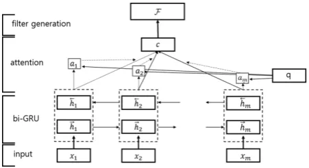
Figure 1 schematically shows the overall architecture of our filter-generating network. The filter-generating network takes an input to a convolution blockI = [x1,x2,· · ·,xm]. mis the

length which can be the number of words in each text or reduced number of it as a result of a pooling operation. Entry xi ∈ Rd is a d-dimensional vector in theithposition in the input.dis equal to the number of filters of the previous convolution block, except for the first convolution block which uses word embedding dimension. It outputs a set ofk convolutional filters F = [f₁,f₂,· · · ,f_k]. Each filterf_i ∈ _Rh·d_{consists of a filter sizehby} dweights.

The filter-generating network generates filters in two phases: context vector generation and filter generation. During context vector generation, the variable size input I is encapsulated into a fixed sizeg-dimensional context vectorc∈_Rg_{. During}

filter generation, the filter-generating network adaptively produces filters from the context vector.

Context Vector Generation We generate a context vector by leveraging the sequential

Figure 1: Graphical illustration of filter-generating network. It generates context vector by self-attending hidden states of bidirectional GRU. Convolutional filters are generated from context vector.

information inherent in inputs. An input to each convolution block is an intermediate hidden representation of a text. Clearly, text has a sequential nature. This property is preserved when text is processed in typical CNNs because they do not shuffle position information between convolution blocks. Operations in CNNs produce an entry for each position from the corresponding position of the filters. As words within a text are dependent on each other, entries within an input are related.

To gain some dependencies between entries in a sequence, we use the Gated Recurrent Unit (GRU) (Cho et al., 2014). We found from our preliminary experiments that GRU shows comparable performance to the Long-Short Term Memory (LSTM) (Hochreiter and Schmidhuber, 1997) with fewer parameters and lower computational cost. We obtain a hidden stateht ∈ Rg for entryxt by concatenating two

hidden states of bidirectional GRU at time stept:

− →

ht= −−−→ GRU(xt,

−−→

ht−1),

←−

ht= ←−−− GRU(xt,

←−−

ht+1),

ht= [ − →

ht; ←−

ht] (1)

We then havemnumber of hidden statesH = [h1,h2,· · · ,hm]. We encapsulateH into a fixed

size context vector c by the weighted sum of hidden states :

c=

m X

j=1

ajhj (2)

calculated as follows:

aj =

exp(q>hj) Pm

k=1exp(q>hk)

(3)

where q is a trainable query vector. This is a special case of self-attention (Lin et al., 2017) with a hop size of one and without a hidden state projection. The context vector c is an effective summarization of the input, and convolutional filters can be readily generated from the fixed size context vector.

Filter Generation : Once we obtain the context vector c by attending hidden states of the bidirectional GRU, we generate convolutional filtersF by a function ofc.

F =f(c) (4)

Although any kinds of function can be applied, we are interested in adding filter-generating networks to existing CNNs. In order for existing CNNs to be trained in an end-to-end fashion even after filter-generating networks are added to them, a differentiable architecture is preferred so that gradients can be backpropagated. We use a fully-connected layer for its simplicity. With this layer, convolutional filters can be generated in two different approaches: full generation andhashed generation. For clarity, we explain how each filter f_i is generated. All filters in F are produced in the same manner.

Full Generation: The most straightforward way to generate a convolutional filter is to use an output of a fully-connected layer directly as a convolutional filter. The layer takes the context vectorcand yields filterf_ias follows:

f_i=Wic (5)

where Wi ∈ R(h·d)×g is the weight matrix for generatingithfilters.

Hashed Generation: Full generation requires numerous parameters because the size of the matrix Wi increases quadratically between the

size of the context vector and the convolutional filter. This may cause a memory issue in very deep CNNs. To address this issue, we employ a hashing trick. The hashing trick allows the filter to be generated with only a fraction of the required number of parameters for full generation.

Our hashing trick is motivated by the recently proposed hash embeddings (Svenstrup et al.,

2017), which constructs word embeddings with the weighted sum of n component vectors from a shared pool. Based on this idea, we generate each f_i by a linear combination of component filtersfrom a shared pool. The shared poolE ∈

Rb×(h·d) containsb component filters. We select

n component filters for f_i from the shared pool using predefined hash functions. The filterf_i is generated by the linear combination as follows:

f_i=

n X

j=1

pi,jHj( ˆfi) (6)

where pi,j is the importance parameter which

determines the weight for the linear combination, and H_j is a function that outputs a component filter from an ID of the filter, which is denoted as ˆ

f_i. H_j is implemented byH_j = E_D

j( ˆfi), where

Dj is a hash function. More specifically,Dj takes

ˆ

f_i, and outputs a bucket index in{1,· · · , b}. The component filter is extracted by taking a row of the bucket index inE. To obtain input-specific filters, we controlpk_i as follows:

pi,j =wi,j>c (7)

where wi,j ∈ Rg is a vector for generating pi,j

from the context vector.

Because we require n numbers of pi,j, n ·g

parameters are needed to generate each filter. The number of the importance parameters n can be chosen to be quite small (we typically use five), and it can provide a huge reduction in the number of parameters compared to the full generation, which uses h ·d·g parameters. The additional parameters for the hashed generation come from the shared poolE. Yet, their portion is relatively small, becauseE is shared across the filters and the size of the shared poolbcan be moderate (we typically use 20).

3.2 Adaptive Convolution

We achieve the adaptive convolution by adding a filter-generating network to each convolution block. The filter-generating network yields filters from its input (output from the previous convolution block). The adaptive convolution involves the input-specifically generated filters, which are applied to inputs to produce new outputs. More formally, a feature

Dataset AG DBPedia Yelp.p Yelp.f Yahoo Amazon.p Amazon.f # of training data 120k 560k 560k 650k 1400k 3600k 3000k # of test data 7.6k 70k 38k 50k 60k 400k 650k

# of classes 4 14 2 5 10 2 5

# of average words 44 54 155 157 108 90 92 # of vocabulary 27k 129k 63k 68k 161k 223k 202k

Table 1: Statistics of the datasets

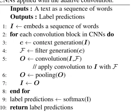
Algorithm 1Generalized forward propagation of CNNs applied with the adative convolution.

Inputs :A text as a sequence of words

Outputs :Label predictions

1: I ←embeds a sequence of words

2: foreach convolution block in CNNsdo

3: c←context generation(I)

4: F ←filter generation(c)

5: O←convolution(I,F)

// apply convolution toI withF 6: O←pooling(O)

7: I ←O

8: end for

9: label predictions←softmax(I)

10: returnlabel predictions

of window in inputs is computed as follows:

oi,j =φ(f>i xj:j+h−1) (8)

where xj:j+h−1 denotes the concatenation of inputs [xj,xj+1,· · ·,xj+h−1], and φ is an activation function such as ReLU (Nair and Hinton, 2010). A position feature oj is

produced by concatenating features from all filters f₁,f₂,· · ·,f_k, which are applied to the jth

position of a window. The output of an adaptive convolution is a sequence of position features O= [o1,o2,· · · ,om−h+1]. This output becomes the input to the next convolution block, after operations predefined in the network structure (such as a pooling) are applied. This procedure is repeated for all convolution blocks in the network. Algorithm1details our approach. Models adopted with our adaptive convolution can be trained in a typical backpropagation, as all components in adaptive convolution are differentiable.

4 Experiments

4.1 Experimental Settings

Datasets and Data Preprocessing We employ seven datasets covering seven different

classification tasks compiled by Zhang et al. (2015). Statistics are summarized in Table 1. ‘AG’,‘DBPedia’ and ‘Yahoo’ are news, ontology, and topic classification datasets, respectively. The others are sentiment classification datasets, where ‘.p’(polarity) in the dataset name indicates that labels are binary and ‘.f’ (full) means that the labels refer to the number of stars.

We tokenize each text using Stanford’s CoreNLP (Manning et al., 2014) after converting all uppercase letters to lowercase letters. In building a vocabulary, we retain words that appear more than five times in a corpus. We replace remaining words with the special ‘UNK’ tokens.

Baselines We select three baseline CNNs to which we apply our adaptive convolution. First one is CNN (Kim, 2014), the basic form of CNNs consists of a single convolution block. The others are recently proposedDPCNN

(Johnson and Zhang,2017) andDenseCNN(Wang et al.,2018b) which employ multiple convolution blocks. We reproduce these three models and apply adaptive convolutions to assess the efficacy of our methodology. All of them are word-level CNNs. We do not apply adaptive convolutions to character-level CNNs (Zhang et al., 2015; Conneau et al., 2017) because of their relatively poor performance compared to word-level CNNs (Johnson and Zhang, 2016). We also compare the performance of our methodology withACNN

(Shen et al., 2018a). Similar to our approach,

Models AG DBPedia Yelp.p Yelp.f Yahoo Amazon.p Amazon.f

CharCNN(Zhang et al.,2015) * 91.45 98.45 95.12 62.05 71.20 95.07 59.57

VDCNN(Conneau et al.,2017) * 91.3 98.7 95.7 64.7 73.4 95.7 63.0

FastText(Joulin et al.,2017) * 92.5 98.6 95.7 63.9 72.3 94.6 60.2

WSEM(Shen et al.,2018b) * 92.66 98.57 95.81 63.79 73.53

LEAM(Wang et al.,2018a) * 92.45 99.02 95.31 64.09 77.42

HAN(Yang et al.,2016) 93.28 98.99 97.08 67.92 75.88 95.94 63.54 (75.8) (63.6)

KnnLSTM(Wang et al.,2017) * 94.2 99.1 94.5 61.9 74.4 95.3 60.3

Self-Attention(Lin et al.,2017)† 91.5 98.3 94.9 63.4 59.8

ACNN(Shen et al.,2018a) 93.82 99.01 96.51 65.98 74.95 95.54 62.03 (98.93) (96.21)

CNN(Kim,2014) 93.15 98.92 96.33 65.52 74.2 95.24 61.09 (93.05) (98.88) (96.54) (65.79) (73.94) (95.73) (62.49) (Ours)AC CNN- full generation 94.07 99.17 97.18 68.12 76.15 96.23 63.60 (Ours)AC CNN- hashed generation 93.81 99.13 97.16 68.07 76.01 96.25 63.74

DPCNN(Johnson and Zhang,2017) 92.87 98.98 96.77 67.01 75.33 96.07 63.30

(Ours)AC DPCNN- full generation 94.03 99.13 97.05 67.91 76.36 96.31 63.94

(Ours)AC DPCNN- hashed generation 93.70 99.10 97.12 67.98 76.07 96.20 63.72

DenseCNN(Wang et al.,2018b) 93.30 99.00 96.48 66.02 74.91 95.95 62.71

(93.6) (99.2) (96.5) (66.0) (63.0) (Ours)AC DenseCNN- full generation 94.35 99.12 97.01 67.63 76.43 96.30 63.91 (Ours)AC DenseCNN- hashed generation 93.63 99.09 96.96 67.74 75.95 96.14 63.59

Table 2: Test accuracies [%] on the seven text classification datasets. Results marked with * are reported in each reference, while results marked with†are re-printed following (Wang et al.,2018b). If not specified, results are from our implementations. Values in the parentheses are from their reference, except forCNNwhose performances is reported in (Johnson and Zhang,2016).

CNN DPCNN DenseCNN

(depth=11) (depth=6)

Baseline 0.4M 3.1M 2.2M

Hashed generation 2.1M 7.1M 11.6M Full generation 217.5M 220M 263.2M

Table 3: Number of parameters in each model. Parameter counts do not include word embeddings.

the models where transfer learning is applied, such as ULMFiT (Howard and Ruder, 2018) to compare the capacity of models by themselves, not the effectiveness of transfer.

Training Details We implement all of the models with PyTorch (Paszke et al., 2017) framework. For all the models and datasets, we use 300 dimensional GloVe (Pennington et al., 2014) vectors trained on 840 billion words for word embedding initialization and initialize out-of-vocabulary words with Gaussian distribution with the standard deviation of 0.6. We do not use the text region embedding (Johnson and Zhang, 2017), for fair comparisons with other comparative models. We optimize parameters using Adam (Kingma and Ba, 2015) with initial learning rate of 0.01 and batch size of 128.

Gradients are clipped at 5.0 by norm. We use ReLU activation after convolution operations.

Model-specific configurations are as follows:

• CNN: We use the total of 300 filters, with 100 filters each having window size of 3,4 and 5.

• DPCNN: We use 100 filters with a size of 3, for each convolution operation. We set the depth to 11 for all the datasets except for the ‘AG’ dataset in which depth is set to 9.

• DenseCNN: We use 75 filters with a size of 3 for each convolution block. Input texts are padded or truncated to a fixed length. We set the fixed length to 300, except for the ‘AG’ in which 100 is used. For ‘AG’ dataset, we use six convolution blocks and seven for all the other datasets.

(a)

(b)

Figure 2: Validation accuracies on Yahoo dataset with different model settings. (a) shows the results with different filter size, where x-axis is in logarithmic scale. (b) illustrates varying performance on different depths.

4.2 Main Results

Table 2 shows the evaluation results on the datasets. In the table, CharCNN and VDCNN

are character level CNNs. FastText, SWEM and

LEAMare word embedding-based models. HAN,

KnnLSTM and Self-Attention are RNN variants. ‘AC’ in the model names indicate that adaptive convolution is applied in the model. Both ‘full generation’ and ‘hashed generation’ are filter-generating methods.

As shown in the table, adaptive convolutions improve all baseline CNNs in all datasets, with no exception. The performance improvements are relatively small for datasets in which known performances are already nearly 100%. In DBPedia dataset, performance improves by as much as 0.15 percentage point (%p) over the baselines. However, for datasets with a potential for considerable performance improvement, such as Yelp.f and Yahoo datasets, adaptive convolutions produce significant results. The performance improvements are up to 2.6%p for Yelp.f dataset.

Without adaptive convolutions, RNNs show better performance than CNNs on most datasets. However, when adaptive convolutions are applied, our baselines perform better than RNN variants on every dataset. Also our approaches perform

(a)

(b)

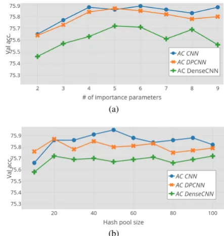
Figure 3: Validation accuracies on Yahoo dataset with different hashed generation settings. (a) shows the results with different number of importance parameters, and (b) depicts performance with different hash (shared) pool size.

better than word embedding-based models except for LEAM model on Yahoo dataset. Furthermore, our adaptive convolutions beat ACNN on all the datasets. This suggests that generating filters block by block with outputs from the previous convolution block is much more efficient than generating filters with original inputs in a single subnetwork.

Adaptive convolutions are found to be effective both in the full and hashed generation. The performance differences between the hashed generation and the full generation are within 0.3%p except for a few cases (AG and Yahoo datasets in DenseCNN). However, the hashed generation is much more efficient than the full generation in terms of the parameter size. Overall, the total number of parameters for models with the hashed generation is less than 3% that of the full generation (Table3).

4.3 Analysis

Analysis on model settings To further demonstrate the effectiveness of our adaptive convolutions, we compare the performance with varying filter sizes and depths. We select CNN

DPCNN and DenseCNN, and their counterparts to which adaptive convolutions are applied. We evaluate the performance with depths ranging from 2 to 13.

The results are illustrated in Figure 2. Note that validation accuracies are lower than test accuracies because only 90% of the training set is used to save remaining 10% for the validation set. As can be seen in the figure, models adopted with our adaptive convolutions show stable performance. In case of filter sizes, CNN

drastically drops performance when the filter size gets smaller. Its performance with the filter size of two is 8.4%p lower than that of the filter size of 100. However, the performance ofAC CNN with the filter size of two declines by 0.6%p from the model with the filter size of 100, which is only 10 percent of the performance loss ofCNN.

This tendency is also found in the analysis

on depths. Performance of DPCNN and

DenseCNN with depths of two or three are 0.6%p lower than that of the baselines with the best performing depths. Contrarily, models with adaptive convolutions perform only 0.12%p lower with depths of two or three than models with the best performing depths.

These results demonstrate that adaptive convolutions effectively generate filters for capturing important information that need to be disambiguated given current inputs. Only few filters and shallow depths are enough for the adaptive convolution to extract such information. This suggests that the required effort to tune hyperparameters can be mitigated by applying adaptive convolutions.

Additional noteworthy fact is that increasing filter sizes and depths beyond a certain level does not lead to performance improvements in all the baseline CNNs. In case of CNN, no change in performance is observed when the filter size exceeds 100. In case of DenseCNN, increasing depths more than seven rather results in a performance drop and increasing depths of

DPCNN exceeding eleven has no effect on the performance. This implies that performance gain is caused by the effectiveness of the proposed adaptive convolution, instead of the increased number of parameters (Table.3).

Analysis on hashed generationWe investigate the effect of the hashed generation settings on the performance with different importance parameters

AC CNN AC DPCNN AC DenseCNN

with GRU 75.86 75.87 75.72 w/o GRU 74.76 75.37 75.36

Table 4: Validation accuracies on Yahoo dataset for the hashed generation-based models with different context generation settings.

and hash (shared) pool sizes. The number of importance parameters is ranging from 2 to 9 and the hash (shared) pool size is in the range from 10 to 100. The results are shown in Figure3. As illustrated, increasing the sizes of hash pool and importance parameters beyond certain threshold does not guarantee performance gain. The number of importance parameter is optimal at five. Higher value of it has no effect on performance and in some cases, negatively affect performance. In case of the hash pool size, 20 is enough for containing candidate filters.

This observation supports the previous finding (Denil et al., 2013) that many redundant parameters exist in deep neural networks. Our results reveal that the networks can be parameterized with a set of candidate weights, and their size can be sufficiently small to significantly reduce the number of required parameters in the network with little performance loss.

Effect of GRU We perform an ablation test to validate the usage of GRUs in generating the context vector. Table 4 shows the results of the ablation test. In all models, utilizing GRUs in generating the context vector significantly

improves performance as much as up to

1.1%p. This clearly indicates the existence of dependencies between entries in each layer. These can be effectively captured and incorporated into the context vector with GRUs and attention-based context vector generation scheme.

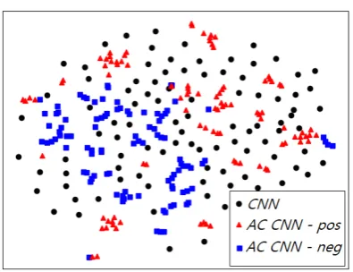
Figure 4: Filters visualized with t-SNE. Filters generated byAC CNN and trained inCNN on Yelp.p dataset are visualized. Negatively and positively labeled samples are used to generate filters from AC CNN.

and the lower left part of the space, respectively. This demonstrates that the generated filters in adaptive convolutions are focused to disambiguate uncertainty in given information. Filters trained inCNN are not specified to given inputs, but are generally tuned to solve given tasks.

5 Conclusion

In this paper, we have introduced the adaptive convolution to endow flexibility to convolution operations. Further, we have proposed the hashing technique which can drastically reduce the number of parameters for adaptive convolutions. We have validated our approach based on the performance evaluation with seven datasets, and investigated the effectiveness of adaptive convolutions through analysis. We believe that our methodology is applicable to other NLP tasks with text pairs, such as textual entailment, question answering. We plan to apply the proposed approach to those tasks in the future.

Acknowledgments

This research was supported by the National Research Foundation of Korea (NRF) funded by the Ministry of Science and ICT (MIST) (No.2018R1A2A1A05078380). This research was also in part supported by the Information Technology Research Center (ITRC) support program supervised by the Institute for Information & communications Technology Promotion (IITP) (IITP-2019-2016-0-00464).

References

Luca Bertinetto, Jo˜ao F Henriques, Jack Valmadre, Philip Torr, and Andrea Vedaldi. 2016. Learning feed-forward one-shot learners. In Proc. of Advances in Neural Information Processing Systems (NIPS), pages 523–531.

Andrei Z Broder, Marcus Fontoura, Evgeniy Gabrilovich, Amruta Joshi, Vanja Josifovski, and Tong Zhang. 2007. Robust classification of rare queries using web knowledge. In Proc. of ACM SIGIR Conference on Research and Development in Information Retrieval (SIGIR), pages 231–238.

Kyunghyun Cho, Bart van Merrienboer, Caglar Gulcehre, Dzmitry Bahdanau, Fethi Bougares, Holger Schwenk, and Yoshua Bengio. 2014. Learning phrase representations using rnn encoder– decoder for statistical machine translation. In

Proc. of Empirical Methods in Natural Language Processing (EMNLP), pages 1724–1734.

Alexis Conneau, Holger Schwenk, Lo¨ıc Barrault, and Yann Lecun. 2017. Very deep convolutional networks for text classification. In European Chapter of the Association for Computational Linguistics (EACL).

Bert De Brabandere, Xu Jia, Tinne Tuytelaars, and Luc V Gool. 2016. Dynamic filter networks. In

Proc. of Advances in Neural Information Processing Systems (NIPS), pages 667–675.

Harm De Vries, Florian Strub, J´er´emie Mary, Hugo Larochelle, Olivier Pietquin, and Aaron C Courville. 2017. Modulating early visual processing by language. In Proc. of Advances in Neural Information Processing Systems (NIPS), pages 6594–6604.

Misha Denil, Babak Shakibi, Laurent Dinh, Nando De Freitas, et al. 2013. Predicting parameters in deep learning. In Proc. of Advances in Neural Information Processing Systems (NIPS), pages 2148–2156.

Vincent Dumoulin, Jonathon Shlens, and Manjunath Kudlur. 2017. A learned representation for artistic style. In International Conference on Learning Representations (ICLR).

David Ha, Andrew Dai, and Quoc V Le. 2017. Hypernetworks. In International Conference on Learning Representations (ICLR).

Sepp Hochreiter and J¨urgen Schmidhuber. 1997. Long short-term memory. Neural computation, 9(8):1735–1780.

Rie Johnson and Tong Zhang. 2016. Convolutional neural networks for text categorization: Shallow word-level vs. deep character-level. arXiv preprint arXiv:1609.00718.

Rie Johnson and Tong Zhang. 2017. Deep pyramid convolutional neural networks for text categorization. In Proc. of Annual Meeting of the Association for Computational Linguistics (ACL), volume 1, pages 562–570.

Armand Joulin, Edouard Grave, Piotr Bojanowski, and Tomas Mikolov. 2017. Bag of tricks for efficient text classification. InProc. of European Chapter of the Association for Computational Linguistics (EACL), volume 2, pages 427–431.

Nal Kalchbrenner, Edward Grefenstette, and Phil Blunsom. 2014. A convolutional neural network for modelling sentences. Proc. of Annual Meeting of the Association for Computational Linguistics (ACL), 1:655–665.

Di Kang, Debarun Dhar, and Antoni Chan. 2017. Incorporating side information by adaptive convolution. In Proc. of Advances in Neural Information Processing Systems (NIPS), pages 3867–3877.

Gabriella Kazai, Iskander Yusof, and Daoud Clarke. 2016. Personalised news and blog recommendations based on user location, facebook and twitter user profiling. In Proc. of ACM SIGIR Conference on Research and Development in Information Retrieval (SIGIR), pages 1129–1132. ACM.

Taesup Kim, Inchul Song, and Yoshua Bengio. 2017. Dynamic layer normalization for adaptive neural acoustic modeling in speech recognition. In Conference of the International Speech Communication Association (INTERSPEECH).

Yoon Kim. 2014. Convolutional neural networks for sentence classification. In Proc. of Empirical Methods in Natural Language Processing (EMNLP), pages 1746–1751.

Diederik P Kingma and Jimmy Ba. 2015. Adam: A method for stochastic optimization. InInternational Conference on Learning Representations (ICLR).

Benjamin Klein, Lior Wolf, and Yehuda Afek. 2015. A dynamic convolutional layer for short range weather prediction. InProc. of IEEE Conference on Computer Vision and Pattern Recognition (CVPR), pages 4840–4848.

Siwei Lai, Liheng Xu, Kang Liu, and Jun Zhao. 2015. Recurrent convolutional neural networks for text classification. In Proc. of AAAI Conference on Artificial Intelligence (AAAI), volume 333, pages 2267–2273.

Jung-Hyun Lee, Jongwoo Ha, Jin-Yong Jung, and SangKeun Lee. 2013. Semantic contextual advertising based on the open directory project.

ACM Transactions on the Web (TWEB), 7(4):24.

Zhouhan Lin, Minwei Feng, Cicero Nogueira dos Santos, Mo Yu, Bing Xiang, Bowen Zhou, and Yoshua Bengio. 2017. A structured self-attentive sentence embedding. In International Conference on Learning Representations (ICLR).

Pengfei Liu, Xipeng Qiu, and Xuanjing Huang. 2017. Dynamic compositional neural networks over tree structure. InProc. of International Joint Conference on Artificial Intelligence, (IJCAI), pages 4054–4060. AAAI Press.

Huma Lodhi, Craig Saunders, John Shawe-Taylor, Nello Cristianini, and Chris Watkins. 2002. Text classification using string kernels. Journal of Machine Learning Research, 2(Feb):419–444.

Laurens van der Maaten and Geoffrey Hinton. 2008. Visualizing data using t-sne. Journal of machine learning research, 9(Nov):2579–2605.

Christopher Manning, Mihai Surdeanu, John Bauer, Jenny Finkel, Steven Bethard, and David McClosky. 2014. The stanford corenlp natural language processing toolkit. InProc. of Annual Meeting of the Association for Computational Linguistics (ACL), pages 55–60.

Vinod Nair and Geoffrey E Hinton. 2010. Rectified linear units improve restricted boltzmann machines. In Proc. of International Conference on Machine Learning (ICML), pages 807–814.

Simon Niklaus, Long Mai, and Feng Liu. 2017. Video frame interpolation via adaptive convolution. In

Proc. of IEEE Conference on Computer Vision and Pattern Recognition (CVPR), pages 670–679.

Hyeonwoo Noh, Paul Hongsuck Seo, and Bohyung Han. 2016. Image question answering using convolutional neural network with dynamic parameter prediction. InProc. of IEEE Conference on Computer Vision and Pattern Recognition (CVPR), pages 30–38.

Aaron van den Oord, Nal Kalchbrenner, Lasse Espeholt, Oriol Vinyals, Alex Graves, et al. 2016. Conditional image generation with pixelcnn decoders. In Proc. of Advances in Neural Information Processing Systems (NIPS), pages 4790–4798.

Adam Paszke, Sam Gross, Soumith Chintala, Gregory Chanan, Edward Yang, Zachary DeVito, Zeming Lin, Alban Desmaison, Luca Antiga, and Adam Lerer. 2017. Automatic differentiation in pytorch. In Advances in Neural Information Processing Systems (NIPS), Workshop.

Ethan Perez, Florian Strub, Harm De Vries, Vincent Dumoulin, and Aaron Courville. 2018. Film: Visual reasoning with a general conditioning layer. In

Proc. of AAAI Conference on Artificial Intelligence (AAAI), pages 3935–3942.

Dinghan Shen, Martin Renqiang Min, Yitong Li, and Lawrence Carin. 2018a. Learning context-sensitive convolutional filters for text processing. InProc. of Empirical Methods in Natural Language Processing (EMNLP), pages 1839–1848.

Dinghan Shen, Guoyin Wang, Wenlin Wang, Martin Renqiang Min, Qinliang Su, Yizhe Zhang, Chunyuan Li, Ricardo Henao, and Lawrence Carin. 2018b. Baseline needs more love: On simple word-embedding-based models and associated pooling mechanisms. In Proc. of Annual Meeting of the Association for Computational Linguistics (ACL), volume 1, pages 440–450.

Dan Tito Svenstrup, Jonas Hansen, and Ole Winther. 2017. Hash embeddings for efficient word representations. In Proc. of Advances in Neural Information Processing Systems (NIPS), pages 4928–4936.

Guoyin Wang, Chunyuan Li, Wenlin Wang, Yizhe Zhang, Dinghan Shen, Xinyuan Zhang, Ricardo Henao, and Lawrence Carin. 2018a. Joint embedding of words and labels for text classification. In Proc. of Annual Meeting of the Association for Computational Linguistics (ACL), volume 1, pages 2321–2331.

Shiyao Wang, Minlie Huang, and Zhidong Deng. 2018b. Densely connected cnn with multi-scale feature attention for text classification. In Proc. of International Joint Conference on Artificial Intelligence, (IJCAI), pages 4468–4474.

Zhiguo Wang, Wael Hamza, and Linfeng Song. 2017. k-nearest neighbor augmented neural networks for text classification. arXiv preprint arXiv:1708.07863.

Yijun Xiao and Kyunghyun Cho. 2016. Efficient character-level document classification by combining convolution and recurrent layers.

arXiv preprint arXiv:1602.00367.

Zichao Yang, Diyi Yang, Chris Dyer, Xiaodong He, Alex Smola, and Eduard Hovy. 2016. Hierarchical attention networks for document classification. In

Proc. of North American Chapter of the Association for Computational Linguistics: Human Language Technologies (NAACL), pages 1480–1489.