Abstract—In this paper, we propose a hybridization of electromagnetism-like mechanism (EM) and particle swarm optimization algorithm (PSO) algorithms to design the proposed functional-link based Petri recurrent fuzzy neural system (FLPRFNS) for application of nonlinear system control. The FLPRFNS has a TSK-type fuzzy consequent part which uses functional-link based orthogonal basis functions and a Petri layer is added to eliminate the redundant fuzzy rule for each input. In addition, the FLPRFNS is trained by a hybrid algorithm- modified EMPSO. The main modification is that the randomly neghiborhoodly local search is replaced by particle swarm optimization algorithm with an instant update particles velocity strategy. Each particle updates its velocity instantaneous- ly one by one and every particle can get best information from system. The modified EMPSO combines the advantages of multipoint search, global optimization, and faster convergence. Simulation results show that the modified EMPSO has the ability of golbal optimization, advantages of faster convergence and FLPRFNS has effect of higher accuracy.
Index Terms—Electromagnetism-like mechanism, particle swarm optimization, functional link, fuzzy neural system, Petri net.
I. INTRODUCTION
Over the decades, a recurrent fuzzy neural network (RFNN) system is proposed to identify and control nonlinear systems [1]. Some other recurrent fuzzy neural systems also have been proposed for nonlinear systems design [2-5]. It has the ability of storing the past information of system. An alternative neural network structure, called functional link neural network (FLNN), has been developed to the well-known multilayer perception network with application to function approximation, pattern recognition and nonlinear channel equalization [6-9]. As the results of [7, 10], using the functional expansion can effectively increase the dimensionality of the input vector and selecting the trigonometric polynomial of orthogonal sine and cosine basis function while there are more than two input signals, the outer product terms would have better convergence results [7]. In order to improve the ability of function approximation
This work was supported in part by the National Science Council,
Taiwan, R.O.C., under contracts NSC-99-2221-E-155-033-MY3.
Ching-Hung Lee is with Department of Electrical Engineering, Yuan-Ze University, Chung-li, Taoyuan 320, Taiwan. (phone: +886-3-4638800, ext: 7119; fax: +886-3-4639355, e-mail: [email protected]).
and have better convergence results, this study uses the functional link neural system to construct the TSK layer. For the last decades, Petri net (PN) has been developed into a powerful tool for modeling, analysis, control, optimization, and implementation of various engineering systems [11-13]. In order to reduce unnecessary compute and eliminate redundant fuzzy rules, we add Petri net into FLPRFNS.
Recently, a novel meta-heuristic based, electromagnetism- like mechanism (EM), for global optimization was proposed [14-18]. EM algorithm is simulated the electromagnetism theory of physics by considering each particle to be an electrical charge. Subsequently, the movement of attraction and repulsion is introduced by Coulomb’s law. Obviously, it has advantages of multiple searches, global optimization, and evaluates many point simultaneously in searching space, they are more likely to find the better solution [16-18]. The particle swarm optimization (PSO) algorithm is easy to implement and has been empirically shown to perform well on many optimization problems [19-23]. Each member in the swarm adapts its search patterns by learning from its own experience and other members’ experiences. In PSO, a member in the swarm, called a particle, each particle has a fitness value and a velocity to adjust its flying direction according to the best experiences of the swarm to search for the global optimum in the solution space. However, a method of updating velocity strategy for PSO algorithm was proposed [22, 23]. In order to improve the performance of EM and enhance its convergent speed, a modified of update particle velocity strategy are adopted in the hybrid electromagnetism-like mechanism and particle swarm optimization algorithms for FLPRFNS designed. The instant update technique is merged into the hybrid algorithm for obtaining a better performance.
The organization of this paper is as follows. Section II introduces FLPRFNS model. Section III introduces hybrid electromagnetism-like and particle swarm optimization algorithms. Section IV shows the simulation results and comparisons. Finally, the conclusion is given
II. FUNCTIONAL-LINK BASED PETRI RECURRENT FUZZY
NEURAL SYSTEM
This section introduces the structure of functional-link neural system (FLNS) and the diagram of the proposed functional-link based Petri recurrent fuzzy neural system (FLPRFNS).
Nonlinear Systems Design by a Novel Fuzzy
Neural System via Hybridization of EM and PSO
Algorithms
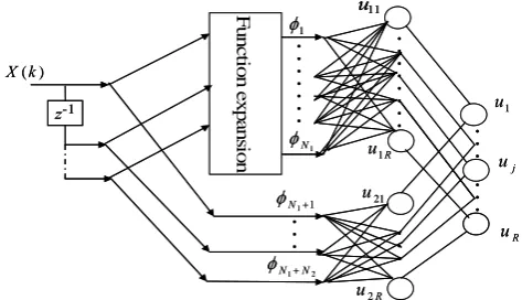
R u2 F u n ct io n e xpa ns io n 1 φ R u1 • • • • • • • • • • • • • • • 1 N φ • • • 1 1+ N
φ u21
2 1 N N+ φ • • • • • • 1 u R u ) (k X z-1 j u • • • 11 u R u2 F u n ct io n e xpa ns io n 1 φ R u1 • • • • • • • • • • • • • • • 1 N φ • • • 1 1+ N
φ u21
[image:2.595.46.283.55.191.2]2 1 N N+ φ • • • • • • 1 u R u ) (k X z-1 j u • • • 11 u11 u
Figure 1: Diagram of combination of functional link neural system and FIR filter: m-dimensional input case. A. Combination of Functional Link Neural System and FIR Filter
A functional expansion block is used to expand the dimension of the input pattern to enhance its representation in a high-dimensional space [6]. Fig. 2 depicts the block diagram of an m-dimensional input for combination of functional link neural system and FIR filter which is a single-layer network and is used for the consequent part of the proposed fuzzy neural system [9]. The FLPRFNS adequately utilizes the FLNS-FIR’s advantages and characteristics of FIR filter to further improve the performance.
Consider an m-dimensional input pattern is defined as
[
]
Tm k
x k x k
X( )= 1( )L ( ) . (1) Every input pattern is contained its past information and assumed there are n-1time delay input is in the form as
X(k)
n m m
m k x k n
x n k x k x × ⎥ ⎥ ⎥ ⎦ ⎤ ⎢ ⎢ ⎢ ⎣ ⎡ + − + − = ) 1 ( ) ( ) 1 ( ) ( 1 1 L M O M L
. (2)
In this paper, we select m=2 to make every input of consequent part is contained its past information. Each set of basis functions for the FLNS-FIR is shown in Fig. 1, where the FLNS-FIR subsection consists of input and trigonometric polynomial basis function. By literature [7], the function expansion block comprises a subset of orthogonal sine and cosine basis functions if there are more than two input signals, it would have better convergence results.
Therefore, the basis functions X1 are defined as
[
]
T m m m m m m T N n k πx n k πx n k x k πx k πx k x n k πx n k πx n k x k πx k πx k x k k X ⎥ ⎥ ⎥ ⎥ ⎥ ⎦ ⎤ ⎢ ⎢ ⎢ ⎢ ⎢ ⎣ ⎡ + − + − + − + − + − + − = = )) 1 ( cos( )) 1 ( sin( ) 1 ( )) ( cos( )) ( sin( ) ( )) 1 ( cos( )) 1 ( sin( ) 1 ( )) ( cos( )) ( sin( ) ( ) ( ) ( 1 1 1 1 1 1 1 1 1 L L L Lφ φ (3) where N1=3×m×n is the number of basis functions from function expansion of input pattern. The linking weights of the FLNS subsection from function expansion X1 isR N R N N R w w w w W × ⎥ ⎥ ⎥ ⎦ ⎤ ⎢ ⎢ ⎢ ⎣ ⎡ = 1 1 11 1 11 1 L M O M L (4)
where R is the rule number of fuzzy neural system. The FIR part of FLNS-FIR consists of basis functions X2
[
T]
m m T N N N n k x k x n k x k x k k X ) 1 ( ) ( ) 1 ( ) ( )] ( ) ( [ 1 1 1
2 1 1 2
+ − + − = = + + L L L Lφ φ (5) where N2=m×n is the number of basis functions for FIR
filter. Similar to the FLNS part, the linking weights of the FIR filter is in the form as
R N R N N N N R N N w w w w W × + + + + ⎥ ⎥ ⎥ ⎦ ⎤ ⎢ ⎢ ⎢ ⎣ ⎡ = 2 2 1 2 1 1 1 ) ( 1 ) ( ) 1 ( 1 ) 1 ( 2 L M O M L (6)
Thus, we define
∑
= = 1 1 1 N i i ij j wu φ (7)
∑
= + + = 2 1 1 1 ) ( ) ( 2 N i i N j i N j wu φ (8) where wij is the corresponding linking weight. Respectively,
j i N
w(1+) is the corresponding link weight of FIR filter and )
(N1+i
φ is the basis past information of input variables. Therefore, the overall output uj of the FLNS is obtained by
uj=λ1×u1j+(1−λ1)×u2j (9)
where λ1 is a convex combination parameter and 1
λ =random(0, 1) which is chosen at initial and is a fixed value. The parameter λ1 in (9) is to make extreme values of
1
λ lead to either a pure FIR or pure FLNS system (λ=1 and λ=0, respectively). If λ1 is set to be a very small initial
value, the occupied place is a transversal filter during training procedure.
1
x xm
) (k X y G 1 − z ij θ
( )2
O Layer 4 Layer 3 Layer 2 Layer 1 G G G G G Π Π ∑
dth dth
j t G dth Π R u2 F u n ct io n e x pa ns io n 1
φ u11
R u1 • • • • • • • • • • • • • • • 1 N φ • • • 1 1+ N
φ u21
2 1N N+
φ••
• • • • 1 u R u j j j u u u 2 1 1 1 ) 1 ( =−××+ λ λ Z-1 j u • • • Layer 5 Layer 6 1
x xm
) (k X y G 1 −
z−1
z
ij
θ
( )2
O Layer 4 Layer 3 Layer 2 Layer 1 G G G G G Π Π ∑
dth dth
j t G dth Π R u2 F u n ct io n e x pa ns io n 1
φ u11
R u1 • • • • • • • • • • • • • • • 1 N φ • • • 1 1+ N
φ u21
2 1N N+
φ••
[image:2.595.309.549.433.597.2]• • • • 1 u R u j j j u u u 2 1 1 1 ) 1 ( =−××+ λ λ Z-1 j u • • • Layer 5 Layer 6
Figure 2: Structure of the proposed FLPRFNS. B. FLPRFNS Structure
A FLPRFNS is depicted in Fig. 2, which uses the FLNS-FIR to form the consequent part. That is, each fuzzy rule corresponds to a sub-FLNS-FIR, comparing a functional link. The FLPRFNS is composed of input layer, membership layer, rule layer, Petri layer, consequent layer and output layer.
Layer 1 (Input Layer): In this layer, each node in this layer is only to transmit input values to the next layer directly, where xi(k), i=1, 2, …, n, represent the input variables.
) ( ) ( ) 1 ( k x k
Layer 2 (Membership Layer): Each fuzzy set Aij here is
described by a Gaussian membership function. Therefore, ( )
( )
(
( )
)
⎥ ⎥ ⎦ ⎤ ⎢
⎢ ⎣
⎡ −
−
= 2
2
2 ( )
exp
ij ij j ij
m k z k
O
σ (11) As above, zj is the fuzzy input linguistic variable,
( )
(
k)
O( )( )
kO
zj ij ij i
1
2 −1⋅ +
= θ , where mij and σij are the mean
and variance of the Gaussian membership function, respectively, of the jth term of the ith input variable xi.
Layer 3 (Rule Layer): Nodes in layer 3 represent rule nodes. The product operator described above is adopted to perform the precondition part of the fuzzy rules. As a result, the output function of each inference node here is
=
∏
i ij
j k O k
O(3)( ) (2)( )
. (12)
) 3 (
j
O represents the firing strength of the corresponding rule. Layer 4 (Petri Layer): Layer 4 is a Petri layer. It is used for producing token makes use of competition laws as follows to select suitable fired nodes:
⎪⎩ ⎪ ⎨ ⎧
< ≥ =
) ( , 0
) ( , 1
) 3 (
) 3 (
th j
th j
j
d k O
d k O
t (13) where tj is the transition and dth is the selected threshold
value which is set between 10-4 ~10-3 to eliminate redundant fuzzy rules as our experience.
Layer 5 (TSK Layer): This layer performs the TSK part by FLNS-FIR. The output of this layer is
⎪⎩ ⎪ ⎨ ⎧
= = ×
=
0 0
1 ) ( )
(
) 3 ( )
5 (
j j j j j
, t
, t k O u k
O (14)
where ujrepresents the jth output of the FLNS. Moreover,
the output nodes of functional link neural network depend on the number of fuzzy rules of the FLPRFNS model.
Layer 6 (Output Layer): The output layer acts as a defuzzifier as
∑
∑
= =
= R
j j R
j j
k O
k O y
1 ) 3 ( 1
) 5 (
) (
) (
(15)
where R is the fuzzy rule number and y is the output of the FLPRFNS.
III. HYBRIDIZATION OF ELECTROMAGNETISM -LIKE AND
PARTICLE SWARM OPTIMIZATION ALGORITHMS
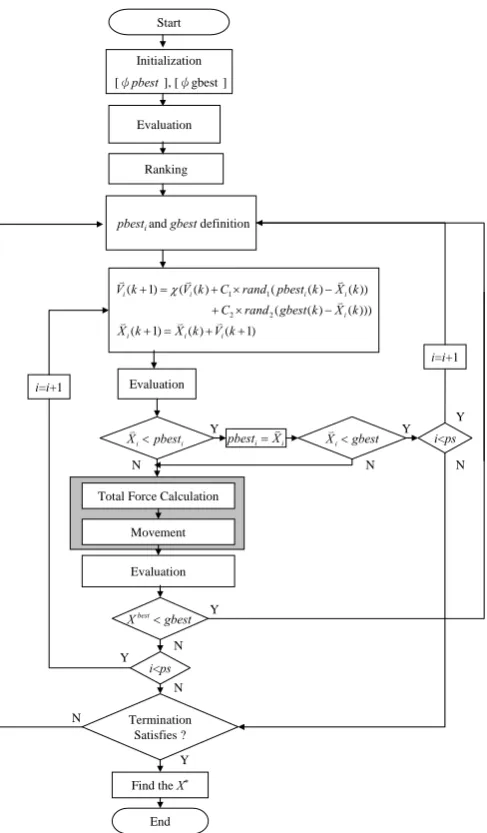
This section introduces the hybrid learning algorithm modified EMPSO for designing FLPRFNS. The modified EMPSO combines the advantages of EM and PSO algorithms to result faster convergence and accuracy. In addition, the instant update concept is implemented in EM and PSO for improving performance. Fig. 3 depicts the flow chart of the modified EMPSO algorithm. Our goal is to use the modified EMPSO to minimize the given cost function by adjusting the link weights in the consequent part and the parameters of the membership functions.
At first, the initial particles are randomly selected from the feasible region of searching space and its initial position and velocity would be set. After initial particle produced, evaluation phase should be done. Each particle is evaluated and ranked by its root-mean-square-error value (RMSE). The particle having smallest RMSE value is selected to be gbest.
After the first generation, each particle’s best individuality and the best particle in whole group would be produced. Started from the second generation, each particle would update its information by using the historical best information. While each particle updates its information, the newest best individual and the newest best particle in group would be obtained. Then, the instant update particles velocity strategy is operated. Detailed description for modified EMPSO is introduced as below.
End Initialization
[ψpbest], [ψgbest ]
Evaluation Start
Ranking
pbestiand gbestdefinition
) 1 ( ) ( ) 1 (
))) ( ) ( (
)) ( ) ( ( ) ( ( ) 1 (
2 2
1 1
+ + = +
− ×
+
− ×
+ = +
k V k X k X
k X k gbest rand C
k X k pbest rand C k V k V
i i i
i i i i
i
v v v
v v v
v
χ
Termination Satisfies ?
Find the X*
Y
N
N
Y Y
i=i+1
i<ps
Y
N
i<ps i=i+1
N
Total Force Calculation
Movement
Evaluation
N
N
Y
gbest Xi<
v Evaluation
i i pbest
Xv< pbesti Xi v
=
Y
[image:3.595.306.550.163.580.2]gbest Xbest<
Figure 3: Flow chart of modified EMPSO algorithm. The EMPSO for optimization problems is in the form of
Minimize f(x)
subject to x∈S, (16) where S {x lk xk uk,lk,uk ,k 1,...,n}
n ≤ ≤ ∈ℜ =
ℜ ∈
= , n is
problem dimension, and f(x) is the objective function, uk and
lk are the corresponding upper bound and lower bound. Each
particle x represents a solution with charge.
Initialization:The modified EMPSO is utilized to find the optimal value
[
m* * * *]
T, ,
Evaluation and Ranking: To evaluate the performance of each particle in training the FLPRFNS controller, we select the root-mean-square-error (RMSE) as realize.
f x e k N N
k
/ ) ( )
(
1 2
∑
=
≡ (17)
where e denotes the approximated error and N denotes the data number.
gbest and pbest Definition:Each particle is evaluated and all particles are ranked and indexed by the corresponding RMSE value. Finally, the particle having the minimal RMSE value is defined as gbest. The current best of particle is also defined.
Local Search for the Modified EMPSO Algorithm: The local search phase is used to gather the local information for each particle xj. In order to reduce the computational complexity, we propose the modified EMPSO to enhance the performance. As shown in Fig. 3, after evaluation phase, each particle will update its velocity and position in local search procedure. Every particle updates its individual information and to be replaced if it has better individuality first. If it has better individuality then it would be substituted and new best individual particle would be produced; if it does not has better individuality then it still use original individual information and did not be updated. After determining of updating individual information or not, the new best individual particle would be determined whether it is used to update the best group particle or not.
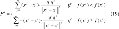
EM Operation- Total Force Calculation:In this phase, a charge is assigned for each particle which is like electromagnetic charge. The charge qi of particle xi is determined by [18]
m i
x f x f
x f x f
q m
k
best worst
best i
i
,..., 2 , 1 , )] ( ) ( [
) ( ) ( exp
1
= ⎥ ⎥ ⎥ ⎥
⎦ ⎤
⎢ ⎢ ⎢ ⎢
⎣ ⎡
− − =
∑
=(18)
As the electromagnetic theory, the force is inversely propositional to the distance between two particles and directly proportional to the product of their particles. Hence, the total force vector exerted on xi computed by the superposition principle as follows
⎪ ⎪ ⎩ ⎪ ⎪ ⎨ ⎧
≥ −
⋅ − −
< −
⋅ − =
∑
∑
≠ ≠
) ( ) ( )
(
) ( ) ( )
(
2 2
i j m
i
j j i
j i i j
i j m
i
j j i
j i i j
i
x f x f if x x
q q x x
x f x f if x x
q q x x
F (19)
After comparing the fitness function values, (i.e., f(x)), the direction of the forces between the particle and the others is selected. For two particles, the one has a better (smaller) fitness value attracts the other one. On the other hand, the particle with larger fitness value repels the others.
EM Operation- Movement: After determining the total force vector Fi, particle xi moves in the direction of the total force by a random step length, i.e.,
RNG F F x
x i
i i i
|| ||
λ
+
= , i=1,2, …, m (20)
⎩ ⎨ ⎧
≤ −
> −
=
0 if ,
0 if ,
i k k i k
i k i k k
F l x
F x u
RNG , k=1,2, …, n (21) where the random step length λ=random (0,1), and RNG is a vector whose components denotes the allowed feasible
movement toward the upper bound, uk,or lower bound lk. The
particle which was not updated in local search phase would be evaluated one by one and the particle has least RMSE value isdefined xbest. The xbest is replaced gbest if its RMSE value is small than gbest and it would become the newest particle and also become the best group particle.
Stop Criterion: In general, the stop criterion can be chosen as maximum generations or specification of control performance in RMSE. In this study, the maximum generations is used to be the stop criterion.
IV. SIMULATION RESULTS
In this example, we consider the tracking control of one-input-one-output nonlinear system and the plant is slightly different from that used in [10]. The plant is described by the different equation
( )
) ( 1
) ( )
1
( 2 u k
k y
k y k
y
p p
p +
+ =
+ (22)
The reference model is described by the following different equation , where
yr(k+1)=0.6yr(k)+r(k) (23)
⎩ ⎨ ⎧
≤ <
≤ +
=
300 100
, ) 25 / 2 sin(
100 ), 25 / 2 sin( ) 10 / 2 sin( ) (
k k
k k
k k
r
π
π π
(24) Note that system state is ypand tracking trajectory vector is yr.
The inputs of FLPRFNS controller are yp and yr and the
output is u. The output of the FLPRFNS controller is the control signal to the plant. The corresponding RMSE function of tracking error is defined
RMSE:
2 / 1 300
1
2
300 / )) 1 ( ) 1 (
( ⎟
⎠ ⎞ ⎜
⎝
⎛
∑
+ − +=
k r p
k y k
y (25)
To show the efficiency and effectiveness of the modified EMPSO, we have the comparison results of EM, PSO, EMPSO and GA algorithms. For the modified EMPSO algorithm, the following parameters are chosen
- Maximum generations: 300 - Particle number: 28 - Control constant: 1 - Positive constant C1: 2
- Positive constant C2: 2
The FLPRFNS’s initial parameters
m
,
σ
,
θ
,
W
1,
W
2 are chosen randomly between [-1, 1] and the network structure is [image:4.595.58.290.549.606.2]- Network structure: 2-10-5-5-5-1 - Parameter number of FLPRFNS: 110 - Rule number of FLPRFNS: 5
Figure 4: The dynamic system control configuration with FLPRFNS controller.
modified EMPSO FLPRFNS
Controller
Nonlinear System u
Σ
yr
yp
e +
-
z-1
modified EMPSO FLPRFNS
Controller
Nonlinear System u
Σ
yr
yp
e +
-
0 50 100 150 200 250 300 -5
-4 -3 -2 -1 0 1 2 3 4 5
Time step
O
ut
put
[image:5.595.326.525.57.192.2]Yr Yp
Figure 5: The system trajectories after 300 generations (solid line: desired trajectory; dashed line: system actual output).
0 50 100 150 200 250 300 0
0.2 0.4 0.6 0.8 1 1.2 1.4 1.6
Generation
RM
S
E
[image:5.595.71.268.59.189.2]FLPRFNS RFNN PRFNN
Figure 6: The comparison results of different network structure with the same number of turning parameters (the
number of turning parameters: 154).
0 50 100 150 200 250 300 0
0.5 1 1.5
FLPRFNS RFNN PRFNN
[image:5.595.82.251.238.366.2]Figure 7: The comparison results of different network structure with the same rule number (rule number: 5).
Table 1: The comparison results of different structure.
Structure. Rule number The number of
turning parameters RMSE
5 35 0.382
9 63 0.351
10 70 0.337
15 105 0.286
16 112 0.273
PRFNN
22 154 0.398
5 35 0.321
9 63 0.296
10 70 0.271
15 105 0.239
16 112 0.225
RFNN
22 154 0.365
3 66 0.233
5 110 0.192
FLPRFNS
7 154 0.152
0 50 100 150 200 250 300
0 0.5 1 1.5
Generation
RM
S
E
mEMPSO EMPSO EM PSO GA
Figure 8: Comparison results of tracking error RMSE (dashed line: modified EMPSO, solid blue line: EMPSO, solid black line: EM, solid pink line: PSO and solid green line:
GA).
0 1000 2000 3000 4000 5000 6000 7000 8000 0
0.2 0.4 0.6 0.8 1 1.2 1.4 1.6 1.8 2
Evaluation
RM
S
E
[image:5.595.327.522.259.384.2]mEMPSO EMPSO EM PSO GA
[image:5.595.91.250.423.547.2]Figure 9: Comparison results in RMSE versus evaluations for Example.
Fig. 4 shows the dynamic system control configuration with FLPRFNS controller and Fig. 5 shows the system trajectories after 300 training cycles of Example: (solid line: desired trajectory; dashed line: system actual output). Fig. 6 shows the comparison results of different network structure with the same number of turning parameters and Fig. 7 shows the comparison results of different network structure with the same rule number. We can observe that whether in the same number of turning parameters or in the same rule number, the FLPRFNS has better training results than RFNN and PFRNN. Detailed comparison results are introduced in Table1. Fig. 8 shows the comparison results of tracking error RMSE for Example: (dashed line: modified EMPSO, solid blue line: EMPSO, solid black line: EM, solid pink line: PSO and solid green line: GA) and Fig. 9 shows the comparison results in RMSE versus evaluations for Example. From Fig. 5, we can observe that the system trajectory is good. Compare with other algorithms are shown in Fig. 8 and Fig. 9. The learning algorithm modified EMPSO has good performance in convergent speed and accuracy.
V. CONCLUSION
[image:5.595.48.291.594.770.2]functional expansion and the consequent part of the proposed FLPRFNS is a nonlinear combination of input variables which enhances the performance of FLPRFNS. Simulation results were presented to show the effectiveness, accuracy and better convergent performance of the FLPRFNS and modified EMPSO algorithm.
REFERENCES
[1] C. H. Lee and C. C. Teng, “Identification and Control of Dynamic
Systems Using Recurrent Fuzzy Neural Networks,” IEEE Trans. on
Fuzzy Systems, Vol. 8, No. 4, pp. 349-366, 2000.
[2] C. J. Lin, C. Y. Lee, and C. C. Chin, “Dynamic Recurrent Wavelet
Network Controllers for Nonlinear System Control,” Journal of The
Chinese Institute of Engineers, Vol. 29, No. 4, pp. 747-751, 2006.
[3] C. J. Lin and Y. J. Xu, “A Novel Evolution Learning for Recurrent
Wavelet-based Neuro-fuzzy Networks,” Soft Computing Journal, Vol.
10, No. 3, pp. 193-205, 2006.
[4] C. F. Juang, “A TSK-type Recurrent Fuzzy Network for Dynamic
Systems Processing by Neural Network and Genetic Algorithms,”
IEEE Trans. on Fuzzy Systems, Vol. 10, No. 2, pp. 155-170, 2002.
[5] P. A. Mastorocostas and J. B. Theocharis, “A Recurrent Fuzzy-neural
Model for Dynamic System Identification,” IEEE Trans. on Systems,
Man, Cybernetics- Part: B, Vol. 32, No. 2, pp. 176-190, 2002.
[6] Y. H. Pao, Adaptive Pattern Recognition and Neural Networks.
Reading, MA: Addison-Wesley, 1989.
[7] J.C. Patra, R.N. Pal, “A functional Link Artificial Neural Network for
Adaptive Channel Equalization,” Expert System with Signal
Processing Vol.43, Issue 2, pp.181-195 May. 1995.
[8] H. Zhao and J. Zhang, “Functional Link Neural Network Cascaded
with Chebyshev Orthogonal Polynomial for Nonlinear Channel Equalization,” ExpertSystemwithSignal Processing Vol. 88, Issue 8, pp. 1946-1957, Aug 2008.
[9] H. Zhao and J. Zhang, “Adaptively Combined FIR and Functional
Link Artificial Neural Network Equalizer for Nonlinear
Communication Channel,” IEEE Trans. on neural network, Vol. 20,
No. 4, pp. 665-674, Apr. 2009.
[10] C. H. Chen, C.J. Lin, and C. T. Lin, “A Functional-Link-Based
Neurofuzzy Network for Nonlinear System Control,” IEEE Trans on
fuzzy systems, Vol. 16, No. 5, pp. 1362-1377, Oct. 2008.
[11] R. David and H. Alla, “Petri Nets for Modeling of Dynamic
Systems—A survey,” Automatica, Vol. 30, no. 2, pp. 175–202, Feb.
1994.
[12] K. Hirasawa, M. Ohbayashi, S. Sakai, and J. Hu, “Learning Petri
Network and Its Application to Nonlinear System Control,” IEEE
Trans.Syst., Man, Cybern., vol. 28, no. 6, pp. 781–789, Dec. 1998.
[13] S. I. Ahson, “Petri Net Models of Fuzzy Neural Networks,” IEEE
Trans.Syst. Man Cybern., vol. 25, no. 6, pp. 926–932, Jun. 1995.
[14] I. Birbil and S. C. Fang, “An Electromagnetism-like Mechanism for
Global Optimization,” Journal of Global Optimization, Vol. 25, No.3, pp. 263-282, 2003.
[15] S. I. Birbil, S. C. Fang, and R. L. Sheu, “On the Convergence of A
Population-based Global Optimization Algorithm,” Journal of Global
Optimization, Vol. 30, No.2, pp. 301-318, 2004.
[16] C. H. Lee and F. K. Chang, “Recurrent Fuzzy Neural Controller
Design for Nonlinear Systems Using Electromagnetism-like
Algorithm,” Far East Journal of Experimental and Theoretical
Artificial Intelligence, Vol. 1, No. 1, pp. 5-22, 2008.
[17] C. H. Lee and Y. C. Lee, “An Improved Electromagnetism-like
Algorithm for Neural Fuzzy Systems Design” Sixteenth session of the
Republic of China on Fuzzy Theory and Its Applications Conference,
Taoyuan, Taiwan, December, 2008.
[18] Ana Maria A. C. Rocha, Edite M. G. P. Fernandes, “On charge effects
to the Electromagnetism-like algorithm,” International Conference
20th EURO Mini Conference “Continuous Optimization and
Knowledge-Based Technologies” May 20–23, 2008, Neringa,
LITHUANIA.
[19] R. C. Eberhart and J. Kennedy, “A new optimizer using particle swarm
theory,” in Proc. 6th Int. Symp. Micromachine Human Sci., Nagoya,
Japan, 1995, pp. 39–43.
[20] J. Kennedy and R. C. Eberhart, “Particle swarm optimization,” in Proc. IEEE Int. Conf. Neural
Networks, 1995, pp. 1942–1948.
[21] Y. Shi and R. C. Eberhart, “A modified particle swarm optimizer,” in
Proc.IEEE Congr. Evol. Comput, pp. 69–73, 1998.
[22] J. J. Liang, A. K. Qin, P. N. Suganthan, and S. Baskar, “Particle swarm optimization algorithms with novel learning strategies,” IEEE Int.
Conf. Systems, Man, Cybernetics, Vol. 4, pp. 3659-3664, The
Netherlands, Oct. 2004.
[23] J. J. Liang, A. K. Qin, “Comprehensive Learning Particle Swarm
Optimizer for Global Optimization of Multimodal Functions, ” IEEE
Trans. on Evolutionary Computation, Vol. 10, No. 3, pp.281-295,