Multidimensional Matrix Mathematics: Notation, Representation, and Simplification, Part 1 of 6

(1)



Abstract—This is the first series of research papers to define multidimensional matrix mathematics, which includes multidimensional matrix algebra and multidimensional matrix calculus. These are new branches of math created by the author with numerous applications in engineering, math, natural science, social science, and other fields. Cartesian and general tensors can be represented as multidimensional matrices or vice versa. Some Cartesian and general tensor operations can be performed as multidimensional matrix operations or vice versa. However, many aspects of multidimensional matrix math and tensor analysis are not interchangeable. Part 1 of 6 defines multidimensional matrix terminology, notation, representation, and simplification.

Index Terms—multidimensional matrix math, multidimensional matrix algebra, multidimensional matrix calculus, matrix math, matrix algebra, matrix calculus, tensor analysis

I. INTRODUCTION

This paper defines a new branch of mathematics called multidimensional matrix mathematics and its new subsets, multidimensional matrix algebra and multidimensional matrix calculus, all three of which were created by the author, Ashu M. G. Solo. This is his first research paper on multidimensional matrix mathematics, multidimensional matrix algebra, and multidimensional matrix calculus. More advanced research papers by Solo on multidimensional matrix math, multidimensional matrix algebra, and multidimensional matrix calculus will soon be published. This paper also shows some applications of multidimensional matrix math.

The classical matrix mathematics [1] that engineering, math, and science students are usually introduced to in college deals with matrices of one or two dimensions. Multidimensional matrix math extends classical matrix math to any number of dimensions. Hence, classical matrix math is a subset of multidimensional matrix math. The classical matrix math taught to many undergraduate college students consists of matrix algebra and matrix calculus whereas multidimensional matrix math consists of multidimensional matrix algebra and multidimensional matrix calculus. To distinguish between the former subjects and latter subjects, matrix math, matrix algebra, and matrix calculus will

Manuscript received March 23, 2010.

Ashu M. G. Solo is with Maverick Technologies America Inc., Suite 808, 1220 North Market Street, Wilmington, DE 19801 USA (phone: (306) 242-0566; email: [email protected]).

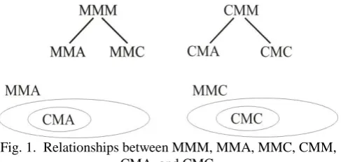
[image:1.595.306.550.418.534.2]

henceforth be referred to as classical matrix math, classical matrix algebra, and classical matrix calculus, respectively. The acronyms CMM, CMA, and CMC, respectively, can be used for these three subjects. The acronyms for multidimensional matrix math, multidimensional matrix algebra, and multidimensional matrix calculus are MMM, MMA, and MMC, respectively. However, for the sake of clarity, these acronyms are not used throughout the text of this research paper. Classical matrix algebra is a subset of multidimensional matrix algebra. Classical matrix calculus is a subset of multidimensional matrix calculus. Therefore, classical matrix algebra and classical matrix calculus are sub-subsets of multidimensional matrix math. The relationships between multidimensional matrix math, multidimensional matrix algebra, multidimensional matrix calculus, classical matrix math, classical matrix algebra, and classical matrix calculus are illustrated in Fig. 1.

Fig. 1. Relationships between MMM, MMA, MMC, CMM, CMA, and CMC.

Some aspects of multidimensional matrix math and tensor analysis [2] are interchangeable. A vector or second order tensor can be represented as a classical matrix, and a classical matrix can be represented as a vector or second order tensor. Similarly, a Cartesian or general tensor of any order can be represented as a multidimensional matrix, and a multidimensional matrix with any number of dimensions can be represented as a Cartesian or general tensor. Some vector or second order tensor operations can be performed as classical matrix math operations, and some classical matrix operations can be performed as vector or second order tensor operations. Similarly, some Cartesian and general tensor operations can be performed as multidimensional matrix math operations, and some multidimensional matrix math operations can be performed as Cartesian or general tensor operations. This is shown in this research paper.

Many aspects of multidimensional matrix math and tensor analysis are not interchangeable. Some vector or second order tensor operations cannot be performed as classical matrix math operations, and some classical matrix operations

Multidimensional Matrix Mathematics:

Notation, Representation, and Simplification,

Part 1 of 6

(2)

cannot be performed as vector or second order tensor operations. Similarly, some Cartesian and general tensor operations cannot be performed as multidimensional matrix math operations, and some multidimensional matrix math operations cannot be performed as Cartesian or general tensor operations. This is shown in this research paper.

Like classical matrix math offers many benefits not present in tensor analysis for a first or second order tensor, multidimensional matrix math offers many benefits not present in tensor analysis for tensors of any order. This is obvious from the description of multidimensional matrix math in this research paper. Similarly, like tensor analysis for a first or second order tensor offers many benefits not present in classical matrix math, tensor analysis for tensors of any order offers many benefits not present in multidimensional matrix math.

The extension of classical matrix math to any number of dimensions has numerous applications in many branches of engineering, math, natural science, social science, and other fields. A few applications are described below. Indeed, Solo needed a multidimensional matrix math for representing the summation of quadratic terms using multidimensional matrices, as described in this series of research papers, to eliminate redundant terms and hence developed this new branch of mathematics. Furthermore, Solo has developed other applications of multidimensional matrix math that could not be done without his multidimensional matrix math. Part 1 of 6 defines multidimensional matrix terminology, notation, representation, and simplification.

II.MULTIDIMENSIONAL MATRIX NOTATION

With multidimensional matrices, instead of simply referring to rows and columns, one refers to dimension 1, dimension 2, dimension 3, and so on or the first dimension, second dimension, third dimension, and so on. The odd dimensions of a multidimensional matrix correspond to rows and the even dimensions correspond to columns.

The number of elements in each of an unlimited number of dimensions can be represented using different variables for each dimension. If a multidimensional matrix has s elements in its first dimension, t elements in its second dimension, u

elements in its third dimension, and v elements in its fourth dimension, it is said to be an s * t * u * v matrix or an s by t by

u by v matrix. Throughout this research paper, the variable s

refers to the number of elements in the first dimension, t refers to the number of elements in the second dimension, u refers to the number of elements in the third dimension, v refers to the number of elements in the fourth dimension, w refers to the number of elements in the fifth dimension, and x refers to the number of elements in the sixth dimension. When there is an indefinite number of dimensions, the number of elements in the final dimension will be represented by the variable z.

Bold uppercase letters, such as A or UNIT, refer to entire multidimensional matrices. The same letters in lowercase with subscripted indices, such as aijk . . . q or unitijk . . . q, refer to

individual elements within the multidimensional matrices. To remain consistent with most descriptions of classical matrix math, commas are not used to separate individual subscripted indices when a single letter is used for each individual subscripted index. However, if two or more letters are used for each individual subscripted index, then commas are

needed to separate individual subscripted indices to avoid confusing the second or third letter of an index as a separate index.

The subscripted indices of a lowercase letter refer to the position of an element within a multidimensional matrix. Each successive index refers to the position within each successive dimension. Throughout this research paper, the index i refers to the position in the first dimension, j refers to the position in the second dimension, k refers to the position in the third dimension, l refers to the position in the fourth dimension, m refers to the position in the fifth dimension, and.

n refers to the position in the sixth dimension. When there is an indefinite number of dimensions, the position in the final dimension will be represented using the index q.

III. MULTIDIMENSIONAL MATRICES

In multidimensional matrix math, a column vector matrix is redefined as a one-dimensional (1-D) matrix with a dimension

s equal to the number of elements in the column vector. In multidimensional matrix math, a row vector matrix is redefined as a two-dimensional (2-D) matrix with dimensions

s * t where s=1 and t is equal to the number of elements in the

row vector. As shown below, this redefinition is necessary, so that the structure of a higher dimensional matrix is evident from the number of elements in each dimension.

A 1-D matrix is a specific case of a 2-D matrix in multidimensional matrix math. Both a 1-D matrix and a 2-D matrix are specific cases of a generalized n-dimensional matrix in multidimensional matrix math.

A submatrix is defined as a lower dimensional matrix

within a higher dimensional matrix. A multidimensional matrix is composed of multiple submatrices with less dimensions, as shown in the following section. Commas are used to separate submatrices in each row of a multidimensional matrix to show that they are not multiplied together.

The term square matrix only applies to 2-D matrices where the number of rows s is equal to the number of columns t. There are no square matrices with one dimension or more than two dimensions.

IV. MULTIDIMENSIONAL MATRIX REPRESENTATION Following is a 1-D matrix with 2 elements:

A = 1 2

a a

     

In a 2-D matrix, there are rows and columns. If a matrix has s

rows and t columns, it is called an s * t matrix. Following is a 2-D matrix with dimensions of 3 * 3:

B =

11 12 13

21 22 23

31 32 33

b b b

 

 

 

Following is a 3-D matrix with dimensions of 2 * 4 * 2:

C =

111 121 131 141

211 221 231 241

112 122 132 142

212 222 232 242

c c c c

  

  

 

 

_ _ 

_ _ 

_ _ 

(3)

This 3-D matrix consists of 2 2-D submatrices.

Following is a 4-D matrix with dimensions of 3 * 2 * 3 * 2:

D =

1111 1211 1112 1212

2111 2211 2112 2212

3111 3211 3112 3212

1121 1221 1122 1222

2121 2221 2122 2222

3121 3221 3122 3222

1131 1231

2131 2231

3131 3231 ,

,

d d d d

d d d d d d                                                1132 1232 2132 2232 3132 3232 , d d d d d d                                 _ _  

This 4-D matrix consists of 6 2-D submatrices. Commas are used to separate 2-D submatrices in each row to show that the 2-D submatrices in each row of the 4-D matrix are not multiplied together.

Following is a 5-D matrix with dimensions of 2 * 2 * 2 * 3 * 2:

E =

11131 12131 11111 12111 11121 12121

21131 22131 21111 22111 21121 22121

11231 12231 11211 12211 11221 12221

21231 22231 21211 22211 21221 22221

1

, ,

e e

e e e e

e e

e e e e

e e

e e e e

e e

e e e e

e                        _ _{ } _ _ _  _ _{ } _ _ _  _ _{ } _{ } _   11132 12132 1112 12112 11122 12122

21132 22132 21112 22112 21122 22122

11232 12232 11212 12212 11222 12222

21232 22232 21212 22212 21222 22222

, ,

e e

e e e

e e

e e e e

e e

e e e e

e e

e e e e

                          _ _{ } _ _ _  _ _{ } _ _ _  _ _{ } _{ } _                           

This 5-D matrix consists of 2 4-D submatrices or 12 2-D submatrices. Commas are used to separate 2-D submatrices in each row to show that the 2-D submatrices in each row of the 4-D submatrices are not multiplied together.

Following is a 5-D matrix with dimensions of 2 * 1 * 2 * 1 * 2:

F =

11111 21111 11211 21211 11112 21112 11212 21212 f f f f f f f f                _ _    _ _    __ _ _                  _ _   _ _   __ _ _  

This 5-D matrix consists of 2 4-D submatrices or 4 1-D submatrices.

Following is a 6-D matrix with dimensions of 2 * 2 * 3 * 2 * 2 * 2:

G =

111111 121111 111211 121211

211111 221111 211211 221211

112111 122111 112211 122211

212111 222111 212211 222211

113111 123111 113211 123211

213111 223111 213211 22321 ,

,

g g g g

                             

111112 121112 111212 121212

211112 221112 211212 221212

112112 122112 112212 122212

212112 222112 212212 222212

113112 123112

1 213112 223112 ,

, ,

g g g g

g g g g                     _ _{ } _   _ _{ } _   _ _{ } _                     113212 123212 213212 223212

111121 121121 111221 121221

211121 221121 211221 221221

112121 122121 112221 122221

212121 222121 212221 222221

113121 , , , g g g g

g g g g

g                                                  

111122 121122 111222 121222

211122 221122 211222 221222

112122 122122 112222 12222

212122 222122

123121 113221 123221

213121 223121 213221 223221

,

, ,

,

g g g g

g g

g g g

g g g g

                    _ _   _ _   _ _                     2 212222 222222

113122 123122 113222 123222

213122 223122 213222 223222 ,

g g

g g g g

                     _ _  _ _  _ _  _ _  _   _  _   _    _ _  __ _{ } _ _  __ _{ } _ _  __ _{ } _ _  

This 6-D matrix consists of 4 4-D submatrices or 24 2-D submatrices. IV. REPRESENTATION OF TENSORS AS MULTIDIMENSIONAL

MATRICES

In tensor analysis, a tensor of order 0 is a scalar, a first order tensor can be represented as a vector or 1-D matrix, and a second order tensor is represented as a 2-D matrix.

In multidimensional matrix math, a tensor of any order (rank) can be represented with a multidimensional matrix in which the order of the tensor is equal to the number of

(4)

V.MULTIDIMENSIONAL MATRIX SIMPLIFICATION The two rules of multidimensional matrix simplification with accompanying examples follow:

1.When the two lowest consecutive dimensions in a multidimensional matrix each have one element, these two consecutive lowest dimensions can be eliminated to create a simplified multidimensional matrix.

The following 4-D matrix with dimensions of 1 * 1 * 2 * 2 can be converted to an equivalent 2-D matrix with dimensions of 2 * 2:

   

1 , 2

3 , 4

 

 

 

= 1 2

3 4

 

 

 

The converse of this rule is two lowest consecutive dimensions with one element in each can be added to a multidimensional matrix to create an equivalent multidimensional matrix.

2. When the highest dimension of a multidimensional matrix has one element, this highest dimension can be eliminated to create a simplified multidimensional matrix.

A 4-D matrix with dimensions of 2 * 2 * 1 * 1 can be converted to a 3-D matrix that looks identical with dimensions of 2 * 2 * 1. This 3-D matrix can be converted to an equivalent 2-D matrix with dimensions of 2 * 2:

5 6

7 8

  

  

 

  =

5 6

7 8

 

 

 

The converse of this rule is that a highest dimension with one element can be added to a multidimensional matrix to create an equivalent multidimensional matrix.

The reason a single lowest dimension with one element can’t be eliminated in a multidimensional matrix is because it would change the layout of elements in the multidimensional matrix to do this. A lowest dimension with one element is significant because this indicates that there is a row vector in a multidimensional matrix. On the other hand, a highest dimension with one element in a multidimensional matrix is not significant and it would not change the layout of elements in the multidimensional matrix if one or more consecutive highest dimensions with one element are eliminated.

VI. DATA REPRESENTATION WITH MULTIDIMENSIONAL MATRICES

In addition to higher order tensors being represented as multidimensional matrices, multidimensional matrices have numerous other applications. Two brief sample applications are described in this section.

Just like classical 2-D matrices can be used to indicate the x-coordinate and y-coordinate of points in 2-D space on a computer screen, multidimensional matrices can be used to indicate the positions of points in multidimensional space. In the following 3-D matrix, wherever there is an element having a value of 1, it indicates that there is a point on a 3-D graph at the x-coordinate equal to the position of this element in the first dimension, at the y-coordinate equal to the position of this element in the second dimension, and at the z-coordinate equal to the position of this element in the third dimension. Different element values could be used to correspond to different colors.

1 1

1

1 1 1

1 1

1

 

 

_ _

 

_ _

_ _

 

 

_ _

_ _

 

This 3-D matrix indicates that there are points at the following integer coordinates on the 3-D graph:

(1, 4, 1), (2, 2, 1), (3, 1, 1), (3, 5, 1), (4, 2, 1), (5, 4, 1), (1, 1, 2), (1, 2, 2), (3, 2, 2), (3, 5, 2), (4, 4, 2), (5, 1, 2), (5, 3, 2), (5, 5, 2), (1, 1, 3), (1, 4, 3), (2, 5, 3), (3, 3, 3), (4, 2, 3), (4, 4, 3), and (5, 2, 3)

Multidimensional matrices can be used to store similar data for different organizations more effectively than classical 2-D matrices. Consider the follow data for students’ standardized exam grades in different engineering departments at different universities:

University of Waterloo

Department of Electrical Engineering

Student Math Grade Physics Grade Software Eng Grade Joe 86 90 79

Nancy 91 82 94 Tim 95 90 99 Department of Mechanical Engineering

Student Math Grade Physics Grade Software Eng Grade Mary 69 52 87

Paul 93 95 97 Tracy 81 79 82 Georgia Institute of Technology

Department of Electrical Engineering

Student Math Grade Physics Grade Software Eng Grade Ron 94 44 87

Jane 91 82 85 Tom 58 51 48 Department of Mechanical Engineering

Student Math Grade Physics Grade Software Eng Grade Jenny 91 79 84

Bob 83 69 97 Ann 75 82 81

(5)

86 90 79 94 44 87

91 82 94 , 91 82 85

95 90 99 58 51 48

69 52 87 91 79 84

93 95 97 , 83 69 97

81 79 82 75 82 81

    

    

_  _{ } _ 

 

   

   

_  _{ } _

 

VII.CONCLUSION

Part 1 of 6 defined multidimensional matrix terminology, notation, representation, and simplification.

Part 2 of 6 defines multidimensional matrix equality as well as the multidimensional matrix algebra operations for addition, subtraction, multiplication by a scalar, and multiplication of two multidimensional matrices. Also, part 2 of 6 describes an alternative representation of the summation of quadratic terms using multidimensional matrix multiplication.

ACKNOWLEDGEMENTS

Madan M. Gupta suggested the idea of developing an algebra of multidimensional matrices. Madan M. Gupta suggested a means of representation for multidimensional matrices. Ashu M. G. Solo modified this means of representation slightly. Then Ashu M. G. Solo fully developed multidimensional matrix algebra and multidimensional matrix calculus, which are described in these research papers (parts 1-6). Also, Ashu M. G. Solo wrote these research papers (parts 1-6).

REFERENCES

[1] Franklin, Joel L. [2000] Matrix Theory. Mineola, N.Y.: Dover. [2] Young, Eutiquio C. [1992] Vector and Tensor Analysis. 2d ed. Boca