Abstract— The various dynamics of the Brusselator chemical reaction and the effect of a sinusoidal force acted on the reaction as a chaotic oscillator has been investigated. In addition, the chaos control in the forced Brusselator oscillator and regulating unstable poles using generalization of the Routh's theorem are the main goals of this work. Likewise, we have regarded chaos as a type of avoided behavior and also as a desired behavior in order to modify the system responses via small perturbation.
Index Terms—Brusselator reaction, Chaos, Control, OGY method, Generalized Routh-Hurwitz criterion.
I. INTRODUCTION
Chaotic oscillations in chemical reactions were discovered in the 1970s first by modelling and then by experiments for the Brusselator models under external action, coupled Brusseltaors, and the Belousov- Zhabotinsky (BZ) [11]. The autocatalytic chemical reaction phenomenon plays an important role for the breakdown of the stability of the thermodynamical branch. In other words, the appropriate types of chemical kinetics show that there is an essential difference between the laws of equilibrium and the laws far from equilibrium. However in far from equilibrium the behavior may become very specific, it permits us to introduce a distinction in the behavior of physical systems which would be incomprehensible in an equilibrium world [8].
The three-variable autocatalator represents chaotic dynamics in an open system structure. This phenomenon emphasizes that one of the essential properties of the chaotic dynamics is their sensitivity to the initial conditions. When a model that includes a dissociation reaction of the autocatalytic species A→X+Y, followed by a recombination reaction
B Y
X+ → , an unusual sensitivity to initial conditions is displayed [3]. Therefore for a chaotic chemical reaction, we need a reaction that guarantees the interaction of the species, and also we should have one (or more) dissociation reaction followed by a recombination reaction. More precisely, a dissociation reaction and a recombination reaction that occur uninterruptedly or after some buffer steps, guarantee the sensitivity to initial conditions. Moreover, the mass action law that affiliates the concentrations of species with respect to time is able to show the time evolution of a chemical reaction.
One of the simple models that is able to exhibit complex Manuscript received February 15, 2010. This work was supported financially by MRL at Qazvin Islamic Azad University, Iran.
Ali Sanayei is an Undergraduate Student in Electrical Engineering. (cell: +98-(0)912-319 81 45; email: [email protected]).
dynamics is the so called "Brusselator" model, which is an example of an autocatalytic oscillating chemical reaction. This model could represent the limit cycle, Andronov-Hopf bifurcation, and also the chaotic behavior when a certain sinusoidal force acts on the system. This force could be created by the heat convection, microwaves, etc, that its behavior is sinusoidal with a small intensity.
Chemical chaos generally corresponds to an unpredictable variation in the concentration of some components that enter an oscillatory reaction [10]. In other words, chaos in a chemical reaction is a nonequilibrium effect that manifests macroscopic scales. It is notable that chaos in chemical reactions is a subtle effect, not easy to see at the one-atom, or one-molecule level. The reason is that the relevant time scales are shorter than a femtosecond. Instead, chaos, an oscillating chemical reaction, and also other systems exhibiting order in macroscopic scales, like a superfluid, or a Bose-Einstein condensate, or a laser manifest in extremely long time-scales (maybe minutes or even more, i.e., slower time scales than those of a single molecule by, at least, 17 powers of 10, and also in very long length scales). Thus, something happens that is a nonequilibrium phase transition, and that makes these systems qualitatively different to those systems that can be described with the well known tools of equilibrium statistical mechanics (i.e., through a partition function) from the knowledge of the molecular structure.
Briefly, chaos in a chemical reaction cannot be connected to atomic or molecular behavior, in the same way as hydrodynamic structure (described e.g., by the Navier-Stokes equation). As an example, waves and turbulence in the ocean cannot be connected to properties of the H2Omolecule. Therefore, the system should be considered as a whole in far from the equilibrium, and in our point of view, the system as a whole is created by the interaction of its components. More precisely, whole is a fuzzy set and the system components are its fuzzy subsets.
Chaotic behavior could be regarded as a dangerous situation for a system. Therefore, the chaos control in this case plays an important role. On the other hand, chaotic behavior is desirable for combustion processes in order to enhance agitation of the air-fuel mix and, consequently, acceleration of the process [11]. In addition, far from the equilibrium may be a source of order. Consequently, the chaos control plays an important role in order to change the system dynamics into the desired situations.
The first control experiment in chemical chaos was carried out in a BZ reaction by the group of Showalter in 1993. The authors applied a map-based, proportional-feedback
Controlling Chaotic Forced Brusselator
Chemical Reaction
algorithm to stabilize periodic behavior in the chaotic regime of an oscillatory BZ reaction. They have also successfully targeted the period-1 orbit in the BZ system [9,10].
The dynamical behaviors of the Brusselator system with periodic and impulsive inputs have been also investigated in 2005 and 2008, respectively [7,15].
In this work, the effect of an external sinusoidal force with small intensity in absence of noise on the dynamics of the Brusselator chemical reaction is investigated. Since the sinusoidal force could perturb the reaction dynamics, accordingly, the goals of this work are controlling chaos using a local feedback control law by linearization of the system's Poincaré map at an unstable periodic orbit (OGY approach), and also, regulating unstable poles using generalization of the Routh's theorem in discrete dynamical systems, instead of a geometrical method that the OGY creators have done.
II. BRUSSELATOR AND FORCED BRUSSELATOR MODEL A. Brusselator Reaction
The mechanism for the classical Brusselator chemical reaction is as follow:
A→k1 X (1)
B+X→k2 Y+D (2)
2X+Y→k3 3X (3)
X→k4 E (4)
This model describes a chemical system that converts a reactant Ato a final product E through four steps and four intermediate species, X,B,Y, and D. Step (2) and (3) are biomolecular, and autocatalytic trimolecular reactions, respectively. Based on the mechanism of Brusselator reaction, product E is resulted from species X in step (4). In addition, species X is the result of steps (1) and (3). These relationships could show the sensitivity to the initial conditions. Denoting the concentrations of A,B,D,E,X, and Y by ], [ ], [ ], [ ], [ ], [A B D E X and [Y], respectively, the evolution of the concentrations of the species as a function of the time t using the mass action law are as follows: [A] k1[A] t =− ∂ ∂ (5)
[B] k2[B][X] t =− ∂ ∂ (6)
[D] k2[B][X] t = ∂ ∂ (7)
[E] k4[X] t = ∂ ∂ (8)
] [ ] [ ] [ ] ][ [ ] [ ] [ 4 2 3 2 1 A B X X Y X X k k k k t = − + − ∂ ∂ (9)
[Y] k2[B][X] k3[X]2[Y] t = − ∂ ∂ (10)
where kj (j=1,2,3,4) is the reaction rate and represented in units of
(
mole .s)
−1. Since the species D and E do not influence the others, therefore, we ignore (7) and (8). Moreover, for simplicity, we suppose that [A] and [B] are maintained constant (i.e., [A]=a, [B]=b, where a,b>0), and all reaction rates kj (j=1,2,3,4) are set equal to unity. Thus, the ordinary differential equations that describe the Brusselator chemical reaction are as follow: − = ∂ ∂ + − + = ∂ ∂ ] [ ] [ ] [ ] [ ] )[ 1 ( ] [ ] [ ] [ 2 2 Y X X Y X Y X X b t b a t (11)The system of ODEs (11) has one fixed point [X]eq =0, and [Y]eq =ba. The Jacobian matrix at the fixed point is obtained as follow: − − − = 2 2 ] [ , ] [ 1 a b a b eq eq Y X J (12)
Consequently, the characteristic polynomial of the Jacobian matrix at the fixed point is λ2+(a2−b+1)λ+a2 =0. (13)
By Routh's theroem [1], the linearized equation in the neighborhood of the fixed point is unstable if and only if
1
2+
>a
b , and is stable if and only if b<a2+1. Therefore, for b>a2+1, we have a limit cycle (see Fig.1).
Assuming b2 =a2+1, an interesting behavior known as Andronov-Hopf bifurcation occurs. It arises when increasing the value of the system's control parameter (µ) stirs two complex conjugate eigenvalues of the Jacobian matrix at
0 =
µ from left-hand side of the imaginary axis to right-hand side in the plane of complex variables [2,12]. Letting
1 2 2 =a +
b , (13) is changed into the following equation:
Fig. 1 Limit cycle behavior in Brusselator chemical reaction.
mole
[image:2.595.284.554.556.750.2]λ2+a2=0 . (14) It is apparent that the eigenvalues of (12) are pure imaginary and nonzero at b2 =a2+1. Moreover, the rate of the real part of the eigenvalues of (12) is nonzero at b2 =a2+1, that is,
{ }
( 1)2 1 2
1
Reλ = tr [ ] ,[ ] = b−a2−
eq eq Y
X
J
{ }
0 2 1 ) 1 (
2 1
Re − 2− = ≠
∂ ∂ = ∂
λ ∂
a b b b
Thus, using the thermodynamic stability criterion or normal mode analysis (e.g., Poincaré-Andronov-Hopf theorem), we could conclude that if b=a2+1, then the Andronov-Hopf bifurcation will be occurred (see Fig.2).
B. Forced Brusselator Reaction
The non-autonomous forced Brusselator chemical reaction is the classical Brusselator system whenever a sinusoidal force with a small intensity acts on it. This sinusoidal force could be created by the heat convection, microwaves, etc, on the reaction, and it could change the reaction kinetics. In other words, the dynamics of the forced Brusselator chemical reaction could be chaotic for certain values of the sinusoidal forcing amplitude.
The non-autonomous system of ordinary differential equations which describes the forced Brusselator chemical reaction is as follow:
− = ∂ ∂
ω +
+ − +
= ∂ ∂
] [ ] [ ] [ ] [
) cos( ]
)[ 1 ( ] [ ] [ ] [
2 2
Y X X Y
X Y
X X
b t
t f b
a t
(15)
where a=[A], b=[B] (a,b>0), [.] shows the concentration of the species, f is the intensity (amplitude) of the sinusoidal force (in units of Newton), and ω is the
angular velocity (in units of rad s).
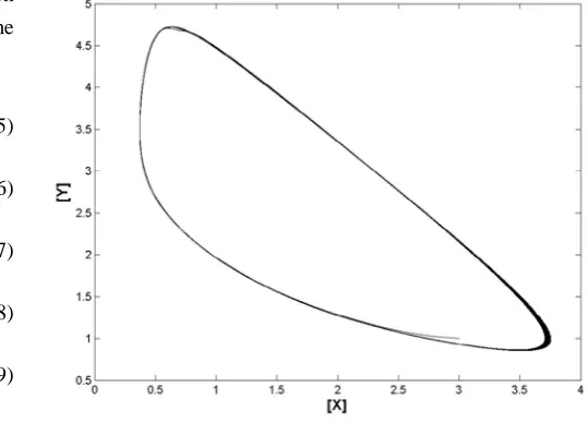
The forced Brusselator system shows the chaotic behavior for a=0.4mole , b=1.2mole , f =0.05 N, and
s rad
81 . 0 =
ω . [7]
Fig.3 shows the forced Brusselator reaction state space and it reveals that the system behavior is chaotic in far-from-equilibrium kinetics (see Fig.3). The far-from-equilibrium concept means that the system does not have an equilibrium point. Instead, it evolves in an equilibrium basin known as the basin of attraction. In addition, since the chaotic dynamics do not have an equilibrium point and they evolve in an equilibrium basin, therefore, a chaotic behavior evolves in far-from-equilibrium. Likewise, it is notable that since the random dynamics do not evolve in an equilibrium basin, thus, the far-from-equilibrium is different from the random dynamics.
III. CHAOS CONTROL
We again consider the system of ODEs that describes the forced Brusselator dynamics (i.e., (15)), where
mole
a=0.4 , b=1.2mole , f =0.05 N, and s
rad
81 . 0 =
[image:3.595.312.553.537.758.2]ω . Our goal in this section is chaos control in the forced Brusselator system using a control method which is based on the local feedback control law by linearization of the system's Poincaré mapping at one unstable periodic orbit (OGY approach). The process of controlling chaos based on OGY method is directed to improving a desired behavior by making only small time-dependent perturbations in an accessible (adjustable) system parameter. The fundamental basis of the OGY approach is that a chaotic attractor has embedded within it an infinite number of unstable periodic orbits [4,5,6,13]. We also regulate the system's unstable poles by generalization of the Routh's theorem. In this context, we consider a new time-dependent value θ(t) where θ(0)=0as follow ( [X]t=0 =0.5mole , and [Y]t=0 =0.2mole ) :
Fig. 2 Andronov-Hopf bifurcation in Brusselator chemical reaction. a=1mole , b=2mole. [X]and [Y] are represented in units of mole .
Fig. 3 State space of thechaotic behavior in forced Brusselator chemical reaction. a=0.4mole , b=1.2mole . [X]and
]
= ∂ θ ∂ − = ∂ ∂ ωθ + + − + = ∂ ∂ 1 ] [ ] [ ] [ ] [ ) cos( ] )[ 1 ( ] [ ] [ ] [ 2 2 t b t f b a t Y X X Y X Y X X (16)
In order to find the fixed points, we should solve simultaneously the following equations:
, 0 ) cos( ] )[ 1 ( ] [ ] [ ] [ 2 = ωθ + + − + = ∂ ∂ f b a
t X Y X
X (17) 0 ] [ ] [ ] [ ]
[ = − 2 =
∂ ∂ Y X X Y b
t . (18) By substituting (18) in (17), we obtain:
a+ f cos(ωθ)−[X]=0 (19) By deriving the both insides of (19) with respect to time, we obtain: 0 ] [ ) sin( = ∂ ∂ − ∂ θ ∂ ωθ ω − t t
f X .
Since =1 ∂
θ ∂
t , and also, 0
] [ = ∂ ∂ t X , therefore, 0 ) sin(ωθ = ω
−f .
Since fω≠0, we could conclude:
ω π =
θm m , m∈ . (20) Substituting (20) in (19), the system's fixed points are as follows:
f
a m
eq ( 1)
]
[X = + − ,
f a b m eq ) 1 ( ] [ − + = Y
By assuming m is an odd number, we obtain the system's fixed point [X]eq =0.35mole , and [Y]eq =3.43mole . We calculate the Jacabian matrix at the fixed point (i.e.,A) and investigate its instability:
− − = − − + − − = 1225 . 0 201 . 1 1225 . 0 201 . 0 ] [ ] [ ] [ 2 ] [ ] [ ] [ 2 1 2 2 eq eq eq eq eq eq b b X Y X X Y X A
The eigenvalues of matrix A are obtained as follow:
347792 . 0 039280 .
0 ±i
=
λ± , i= −1
Since Re{λ±}>0, therefore, we conclude that the computed fixed point is unstable. Based on the OGY fundamental basis (i.e., an infinite number of unstable periodic orbits are embedded in the chaotic attractor), we consider a linear approximation for the forced Brusselator system's Poincaré map at the computed unstable fixed point. We assume that the magnitude of the sinusoidal force (i.e., f ) is the system's accessible control parameter and it could be perturbed in close of a nominal value (i.e., f =0.05 N).
In addition, we assume that the system is chaotic at f = f . We calculate the matrix Bwhich is a column vector and defined as a partial derivative with respect to the system's control parameter at the unstable fixed point:
− = 0 1 B
The controllability matrix Cis calculated as follow: − − = ≡ 201 . 1 0 201 . 0 1 ] [B AB
C
Since matrix C is 2×2, and det(C)≠0, therefore,RankC=dim(ImC)=2. Thus, based on the uniqueness theorem, the pole placement problem has a unique solution [5].
Grebogi, et al. assumed a linear approximation for the system's Poincaré mapping in neighborhood of an unstable periodic orbit and control parameter [6,5]. By considering the following discrete-time dynamical system
) , (
1 F i f
i = Ψ
Ψ+ ,
we could approximate it based as follow:
Ψi+1−Ψeq(f)=[A−BKT][Ψi−Ψeq(f)] (21) where Ψi∈n
and F is sufficiently smooth in both variables and f (the magnitude of the sinusoidal force) is the control parameter. Matrix KT, and consequently, matrix
T BK
A− (regulator matrix) are calculated so as to regulate the unstable periodic orbit. By applying the pole placement technique, the regulator matrix will be found as follow:
− − + + − = − 1225 . 0 201 . 1 832639 . 0 48626 . 0 1225 . 0 201 .
0 k1 k1 k2
T
BK A
where k1 and k2 are real numbers and they should be computed so as to regulate the unstable fixed point. The characteristic polynomial of the regulator matrix is obtained as follow:
λ2+σ1λ+σ2 =0 (22) where
0785 . 0
1 1= −
σ k , and
1225 . 0 706498 . 0 999999 .
0 2 1
2 = + +
σ k k .
The last stage of the pole placement technique is finding 1
k and k2 in order to stabilize the unstable fixed point. In other words, the eigenvalues of the regulator matrix must be smaller than unity. Since we do not deal with some ODEs, therefore the applying Routh's theorem is not sufficient in this case. In this regard, we define a mapping from inside of the circle centered at zero with radius unity into the negative half plane of the complex variables where the real parts of the numbers are negative. By using this trick, we can use the Routh's theorem in discrete dynamical systems in order to stabilize the system's unstable poles. Substituting the following mapping, that is,
1 1 − ϕ + ϕ λ
0 1 1
1 2 2
2 1
2 1 2
1 2
2 =
+ σ + σ
σ + σ − + ϕ + σ + σ
σ − +
ϕ . (23)
Based on the Routh's theorem [1], the real parts of the roots of (23) are negative if and only if
> + σ + σ
σ + σ −
> + σ + σ
σ −
. 0 1 1
, 0 1 2 2
2 1
2 1
2 1
2
(24)
For instance, σ1 =−0.40 and σ2 =0.03 satisfy the inequalities (24). Therefore, the regulator matrix is obtained as follow:
− −
= −
1225 . 0 2010 . 1
0786 . 0 5225 . 0 T BK
A (25)
By substituting (25) in (21), the linearized Poincaré mapping for the forced Brusselator chemical reaction will be found:
− −
− −
=
− −
+ +
43 . 3 ] [
35 . 0 ] [ 1225 . 0 2010 . 1
0786 . 0 5225 . 0 43 . 3 ] [
35 . 0 ] [
1 1
i i
i i
Y X Y
X
(26)
Equation (26) contains two mappings that they exhibit the control procedure. In addition, Fig.4 shows the result of control action on the system. As seen, by adjusting the control parameter in neighborhood of the nominal value, the unstable fixed point that is embedded in the chaotic forced Brusselator chemical reaction has been stabilized.
The chaotic dynamics could be considered as an avoided behavior. This hypothesis could be acceptable in the cases that the human activities are not able to adapt themselves with nature. For instance, the temperature difference between two layers of fluid creates some counter-rotating vortices. If a rigid body moves between these layers, since it is not able to adapt itself with this chaotic behavior, therefore, this behavior could be dangerous for its structure. If we suppose this situation (i.e., chaos as an avoided behavior) in forced Brusselator system, we should eliminate the effect of the chaotic behavior source (i.e., the sinusoidal forcing). In this regard, we could radiate an electromagnetic ray, or add a catalyst for eliminating the sinusoidal forcing. Assuming that the adjustable system control parameter is the forcing frequency, the behavior of the electromagnetic ray should be sinusoidal that its intensity is f and its angular velocity is
ω −
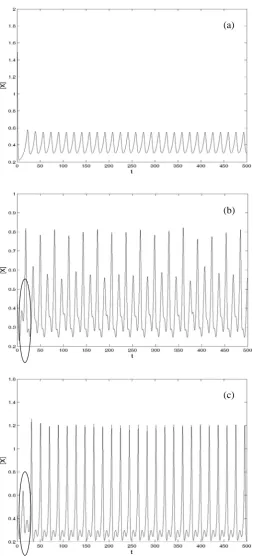
π . By rating this ray to the forced Brusselator system, we could omit the effect of sinusoidal force. Consequently, the forced Brusselator reaction behavior will not be chaotic and it will be periodic as seen in Fig. 5(a).
Another, perhaps more positive view, of the opportunities provided by chaos control is to imagine that we have a chemical reactor set up and operating under a standard set of operating conditions (e.g., flow rates, input concentrations, etc) and we want to be able to modify the response via small perturbations of those operating conditions in a way that slightly different perturbations lead to significantly different responses (all periodic orbits that are embedded in the chaotic attractor). In this case, the chaos control approach is one that might be easily realizable in practice. In other words, by using any accessible parameter, we are able to modify the chaotic behavior and change the system dynamics into a desired periodic orbit. In the forced Brusselator system, we supposed that the sinusoidal forcing amplitude is the accessible parameter (likewise, we could choose the frequency as an accessible parameter as the previous case). It is notable that we could vary the control parameter while it is restricted to lie in some small interval. For instance, By considering that the forcing amplitude is the system adjustable control parameter and the frequency is fixed, if we choose f =0.04 N, we could have a periodic behavior as seen in Fig.5(b). By considering that the frequency is the adjustable control parameter and the forcing amplitude is fixed, if we choose
s rad
65 . 0 =
[image:5.595.31.295.472.786.2]ω , we could have another periodic behavior as seen in Fig.5(c). It should be noted that one control parameter that obeys the controllability condition is enough for adjusting and controlling chaos. The control procedure is activated only if Ψi satisfies the conditions that the system control parameter lies in a small interval. Since nonlinearity is not included in the linearized system's Poincaré mapping, the control procedure may not be able to bring the orbit to the stabilized fixed point. Interestingly, since the orbit on the uncontrolled chaotic attractor is ergodic [5], therefore, the control parameter limitation is satisfied after some time. This chaotic transient is observable in Fig.5(b) and Fig.5(c). Moreover, Romeiras, et al. discussed that the distribution of chaotic transient lengths of such chaotic transient depends sensitively on the random initial conditions in the basin of Fig. 4 Stability of the unstable periodic orbit in the chaotic forced
Brusselator system. [X]eq =0.35mole , and
mole eq 3.43
]
[Y = . The horizontal axis shows the iteration numbers, and the vertical axis shows the concentration of X and
Y
.eq
] [X
eq
attraction and it will be exponential [5]. Consequently, the probability that the time is chosen in the basin of attraction to achieve control is obtained as follow:
τ
τ τ − τ =
∫
τ
d
P 1 exp
where τ is the average time to achieve control.
IV. CONCLUDING REMARKS
The aims of this work were investigation and control of a chemical chaotic oscillation known as forced classic Brusselator reaction. The control procedure was done using the OGY method. The regulating unstable periodic orbit which had been embedded in the chaotic attractor was done using generalization of the Routh's theorem. We also considered two cases for chaos control: first, chaos as an avoided behavior, and second, chaos as a desired behavior. The first assumption is acceptable when the human activities are not able to adapt themselves with nature, and the second assumption is important in order to modify the system dynamics. In the last section, we emphasized that because of nonlinearity, we have a chaotic transient to achieve the control procedure. Interestingly, Tél presented a method for the controlling transient chaos [14].
ACKNOWLEDGMENT
In memory of my dear cousin: Hosein. It is my pleasure to dedicate this paper to my darling and nice sisters: Somayeh, and Sahar. Likewise, the author is really thankful to Prof. C. Grebogi, M. Matias, and S. Scott for very helpful discussions in controlling chaos and chaotic chemical reactions.
REFERENCES
[1] E. Hairer, S.P. Nrsett, and G. Wanner, “Stability; Periodic solutions, limit cycles, strange attractors (Solving Ordinary Differential Equations I – Nonstiff Problems),” 2nd ed., Germany: Springer, 2000, pp. 80-91, 111-128.
[2] N. A. Magnitskii, and S. V. Sidrov, “Bifurcations in nonlinear systems of ordinary differential equations (New Methods For Chaotic Dynamics),” 1st ed., vol. 58, Singapore: World Scientific, 2006, pp. 50-74.
[3] J. Wang, H. Sun, S. K. Scott, and K. Showalter, “Uncertain dynamics in nonlinear chemical reactions,” Phys. Chem. Chem. Phys., No. 5, 2003, pp. 5444-5447.
[4] I. R. Epstein, K. Showalter, “Nonlinear Chemical Dynamics: Oscillations, Patterns, and Chaos,” J. Phys. Chem., No. 100, 1996, pp. 13132-13147.
[5] F. J. Romeiras, C. Grebogi, E. Ott, and W. P. Dayawansa, “Controlling chaotic dynamical systems,” Physica D, No. 58, 1992, pp. 165-192.
[6] C. Grebogi, Y. -C. Lai, “Controlling chaotic dynamical systems,” Systems & Control Lett., No. 31, 1997, pp. 307-312.
[7] I. Bashkirtseva, and L. Ryashko, “Sensitivity and chaos control for the forced nonlinear oscillations,” Chaos, Solitons and Fractals, No. 26, 2005, pp. 1437-1451.
[8] I. Prigogine, “Time, Structure, and Fluctuations,” Nobel Lecture, December 1977.
[9] V. Petrov, V. Gáspár, J. Masere, and K. Showalter, “Controlling chaos in the Belousov-Zhabotinsky reaction,” Nature, vol. 361, 1993, pp. 240-243.
[10] S. Boccaletti, C. Grebogi, Y. -C. Lai, H. Mancini, and D. Maza, “The control of chaos: Theory and applications,” Physical Reports, No. 329, 2000, pp. 103-197.
[11] B. R. Andrievskii, and A.L. Fradkov, “Control of chaos: Methods and Applications. II. Applications,” Automation and Remote Control, No. 4, 2004, pp. 3-34.
[12] M. P. McDowell, “Mathematical modeling of the Brusselator,” unpublished.
[13] J. Kurths, S. Boccaletti, C. Grebogi, and Y. -C. Lai, “Introduction: Control and synchronization in chaotic dynamical systems,” Chaos, vol. 13, No. 1, 2003, pp. 126-127.
[14] T. Tél, “Controlling transient chaos,” J. Phys. A, No. 24, 1991, L1359-68.
[image:6.595.36.291.145.703.2][15] M. Sun, Y. Tan, L. Chen, “Dynamical behaviors of the brusselator system with impulsive input,” J. Math. Chem., No. 44, 2008, pp. 637-649.
Fig. 5 The result of chaos control (as an avoided behavior) to a periodic behavior (a), The result of chaos control to a periodic orbit by assuming that the forcing amplitude is the control parameter (b), The result of chaos control to a periodic orbit by assuming that the frequency is the control parameter (c). The time series in the restricted area in (b) and (c) are the chaotic transient. They also determine the time to achieve control.
(a)
(b)
![Fig. 2 Andronov-Hopf bifurcation in Brusselator chemical a=1moleb=2mole[X][Y]](https://thumb-us.123doks.com/thumbv2/123dok_us/1303075.660014/3.595.312.553.537.758/fig-andronov-hopf-bifurcation-brusselator-chemical-moleb-mole.webp)
![Fig. 4 Stability of the unstable periodic orbit in the chaotic forced [X]=.035mole](https://thumb-us.123doks.com/thumbv2/123dok_us/1303075.660014/5.595.31.295.472.786/fig-stability-unstable-periodic-orbit-chaotic-forced-mole.webp)