Length bias in Encoder Decoder Models and a Case for Global Conditioning
Pavel Sountsov Google
Sunita Sarawagi∗
IIT Bombay [email protected]
Abstract
Encoder-decoder networks are popular for modeling sequences probabilistically in many applications. These models use the power of the Long Short-Term Memory (LSTM) archi-tecture to capture thefull dependenceamong variables, unlike earlier models like CRFs that typically assumed conditional independence among non-adjacent variables. However in practice encoder-decoder models exhibit a bias towards short sequences that surprisingly gets worse with increasing beam size.
In this paper we show that such phenomenon is due to a discrepancy between the full sequence margin and the per-element margin enforced by the locally conditioned training objective of a encoder-decoder model. The discrepancy more adversely impacts long sequences, explaining the bias towards predicting short sequences. For the case where the predicted sequences come from a closed set, we show that a glob-ally conditioned model alleviates the above problems of encoder-decoder models. From a practical point of view, our proposed model also eliminates the need for a beam-search dur-ing inference, which reduces to an efficient dot-product based search in a vector-space.
1 Introduction
In this paper we investigate the use of neural net-works for modeling the conditional distribution
Pr(y|x)over sequencesyof discrete tokens in
re-sponse to a complex inputx, which can be another ∗ Work done while visiting Google Research on a leave from IIT Bombay.
sequence or an image. Such models have applica-tions in machine translation (Bahdanau et al., 2014; Sutskever et al., 2014), image captioning (Vinyals et al., 2015), response generation in emails (Kannan et al., 2016), and conversations (Khaitan, 2016; Vinyals and Le, 2015; Li et al., 2015).
The most popular neural network for probabilis-tic modeling of sequences in the above applications is the encoder-decoder (ED) network (Sutskever et al., 2014). A ED network first encodes an inputx
into a vector which is then used to initialize a re-current neural network (RNN) for decoding the out-puty. The decoder RNN factorizesPr(y|x)using
the chain rule as QjPr(yj|y1, . . . , yj−1,x) where
y1, . . . , yn denote the tokens in y. This factoriza-tion does not entail any condifactoriza-tional independence assumption among the{yj} variables. This is un-like earlier sequence models un-like CRFs (Lafferty et al., 2001) and MeMMs (McCallum et al., 2000) that typically assume that a token is independent of all other tokens given its adjacent tokens. Modern-day RNNs like LSTMs promise to capture non-adjacent and long-term dependencies by summarizing the set of previous tokens in a continuous, high-dimensional state vector. Within the limits of parameter capacity allocated to the model, the ED, by virtue of exactly factorizing the token sequence, is consistent.
However, when we created and deployed an ED model for a chat suggestion task we observed sev-eral counter-intuitive patterns in its predicted outputs. Even after training the model over billions of exam-ples, the predictions were systematically biased to-wards short sequences. Such bias has also been seen in translation (Cho et al., 2014). Another curious
phenomenon was that the accuracy of the predictions sometimes dropped with increasing beam-size, more than could be explained by statistical variations of a well-calibrated model (Ranzato et al., 2016).
In this paper we expose a margin discrepancy in the training loss of encoder-decoder models to ex-plain the above problems in its predictions. We show that the training loss of ED network often under-estimates the margin of separating a correct sequence from an incorrect shorter sequence. The discrepancy gets more severe as the length of the correct sequence increases. That is, even after the training loss con-verges to a small value, full inference on the training data can incur errors causing the model to be under-fitted for long sequences in spite of low training cost. We call this the length bias problem.
We propose an alternative model that avoids the margin discrepancy by globally conditioning the
P(y|x)distribution. Our model is applicable in the many practical tasks where the space of allowed out-puts is closed. For example, the responses gener-ated by the smart reply feature of Inbox is restricted to lie within a hand-screened whitelist of responses
W ⊂ Y(Kannan et al., 2016), and the same holds for
a recent conversation assistant feature of Google’s Allo (Khaitan, 2016). Our model uses a second RNN encoder to represent the output as another fixed length vector. We show that our proposed encoder-encoder model produces better calibrated whole se-quence probabilities and alleviates the length-bias problem of ED models on two conversation tasks. A second advantage of our model is that inference is significantly faster than ED models and is guaran-teed to find the globally optimal solution. In contrast, inference in ED models requires an expensive beam-search which is both slow and is not guaranteed to find the optimal sequence.
2 Length Bias in Encoder-Decoder Models
In this section we analyze the widely used encoder-decoder neural network for modelingPr(y|x)over
the space of discrete output sequences. We use
y1, . . . , ynto denote the tokens in a sequencey. Each yiis a discrete symbol from a finite dictionaryV of sizem. Typically,mis large. The lengthnof a
se-quence is allowed to vary from sese-quence to sese-quence even for the same inputx. A special token EOS∈V
is used to mark the end of a sequence. We useYto denote the space of such valid sequences and θto
denote the parameters of the model.
2.1 The encoder-decoder network
The Encoder-Decoder (ED) network represents
Pr(y|x, θ)by applying chain rule to exactly factor-ize it asQn
t=1Pr(yt|y1, . . . , yt−1,x, θ). First, an
en-coder with parametersθx ⊂θis used to transform xinto ad-dimensional real-vectorvx. The network used for the encoder depends on the form ofx —
for example, whenxis also a sequence, the encoder
could be a RNN. The decoder then computes each
Pr(yt|y1, . . . , yt−1,vx, θ)as
Pr(yt|y1, . . . , yt−1,vx, θ) =P(yt|st, θ), (1)
wherestis a state vector implemented using a recur-rent neural network as
st= (
vx ift= 0,
RNN(st−1, θE,yt−1, θR) otherwise.
(2)
where RNN() is typically a stack of LSTM cells that captures long-term dependencies,θE,y ⊂θare pa-rameters denoting the embedding for tokeny, and θR⊂θare the parameters of the RNN. The function
Pr(y|s, θy)that outputs the distribution over them tokens is a softmax:
Pr(y|s, θ) = e
sθS,y
esθS,1 +. . .+esθS,m, (3) whereθS,y ⊂θdenotes the parameters for tokenyin the final softmax.
2.2 The Origin of Length Bias
The ED network builds a single probability distri-bution over sequences of arbitrary length. For an input x, the network needs to choose the highest
probability yamong valid candidate sequences of
widely different lengths. Unlike in applications like entity-tagging and parsing where the length of the output is determined based on the input, in appli-cations like response generation valid outputs can be of widely varying length. Therefore,Pr(y|x, θ)
finite, we show that the ED model is biased against long sequences. Other researchers (Cho et al., 2014) have reported this bias but we are not aware of any analysis like ours explaining the reasons of this bias.
Claim 2.1. The training loss of the ED model under-estimates the margin of separating long sequences from short ones.
Proof. Let x be an input for which a correct
out-put y+ is of length ` and an incorrect output y−
is of length 1. Ideally, the training loss should put a positive margin between y+ and y− which
islog Pr(y+|x)−log Pr(y−|x). Let us investigate
if the maximum likelihood training objective of the ED model achieves that. We can write this objective as:
max
θ log Pr(y
+ 1|x, θ)+
` X
j=2
log Pr(yj+|y1+...j−1,x, θ).
(4) Only the first term in the above objective is in-volved in enforcing a margin between y+ and y− because log Pr(y1+|x) is maximized when log Pr(y−1|x) is correspondingly minimized. Let mL(θ) = log Pr(y1+|x, θ) − log Pr(y1−|x, θ), the
local margin from the first position and mR(θ) = P`
j=2log Pr(y+j |y1+...j−1,x, θ). It is easy to see
that our desired margin between y+ and y− is
log Pr(y+|x) −log Pr(y−|x) = mL+mR. Let mg =mL+mR. Assuming two possible labels for the first position (m = 2)1, the training objective in Equation 4 can now be rewritten in terms of the margins as:
min
θ log(1 +e
−mL(θ))−m
R(θ)
We next argue that this objective is not aligned with our ideal goal of making the global marginmL+mR positive.
First, note thatmRis a log probability which un-der finite parameters will be non-zero. Second, even though mL can take any arbitrary finite value, the training objective drops rapidly whenmLis positive. When training objective is regularized and training data is finite, the model parameters θ cannot take
1For m > 2, the objective will be upper bounded by
minθlog(1 + (m−1)e−mL(θ))−mR(θ). The argument that
follows remains largely unchanged
very large values and the trainer will converge at a small positive value ofmL. Finally, we show that the value ofmRdecreases with increasing sequence length. For each positionjin the sequence, we add
tomRlog-probability ofy+j . The maximum value oflog Pr(yj+|y+1...j−1,x, θ)islog(1−)whereis
non-zero and decreasing with the magnitude of the parameters θ. In general, log Pr(y+j |y+1...j−1,x, θ)
can be a much smaller negative value when the input
xhas multiple correct responses as is common in
con-versation tasks. For example, an input likex=‘How
are you?’, has many possible correct outputs:y∈{‘I
am good’, ‘I am great’, ‘I am fine, how about you?’, etc}. Letfj denote the relative frequency of output y+j among all correct responses with prefixy+1...j−1.
The value ofmRwill be upper bounded as
mR≤ ` X
j=2
log min(1−, fj)
This term is negative always and increases in mag-nitude as sequence length increases and the set of positive outpus have high entropy. In this situation, when combined with regularization, our desired mar-ginmgmay not remain positive even thoughmLis positive. In summary, the core issue here is that since the ED loss is optimized and regularized on the lo-cal problem it does not control for the global, task relevant margin.
This mismatch between the local margin optimized during training and the global margin explains the length bias observed by us and others (Cho et al., 2014). During inference a shorter sequence for which
mRis smaller wins over larger sequences.
This mismatch also explains why increasing beam size leads to a drop in accuracy sometimes (Ran-zato et al., 2016)2. When beam size is large, we are more likely to dig out short sequences that have oth-erwise been separated by the local margin. We show empirically in Section 4.3 that for long sequences larger beam size hurts accuracy whereas for small sequences the effect is the opposite.
2.3 Proposed fixes to the ED models
Many ad hoc approaches have been used to alleviate length bias directly or indirectly. Some resort to
nor-2Figure 6 in the paper shows a drop in BLEU score by 0.5 as
malizing the probability by the full sequence length (Cho et al., 2014; Graves, 2013) whereas (Abadie et al., 2014) proposes segmenting longer sentences into shorter phrases. (Cho et al., 2014) conjectures that the length bias of ED models could be because of limited representation power of the encoder network. Later more powerful encoders based on attention achieved greater accuracy (Bahdanau et al., 2014) on long sequences. Attention can be viewed as a mechanism of improving the capacity of the local models, thereby making the local marginmLmore definitive. But attention is not effective for all tasks — for example, (Vinyals and Le, 2015) report that
attention was not useful for conversation.
Recently (Bengio et al., 2015; Ranzato et al., 2016) propose another modification to the ED training ob-jective where the true tokenyj−1 in the training term
log Pr(yj|y1, . . . , yj−1) is replaced by a sample or
top-k modes from the posterior at positionj−1via
a careful schedule. Incidently, this fix also helps to indirectly alleviate the length bias problem. The sam-pling causes incorrect tokens to be used as previous history for producing a correct token. If earlier the incorrect token was followed by a low-entropy EOS token, now that state should also admit the correct token causing a decrease in the probability of EOS, and therefore the short sequence.
In the next section we propose our more direct fix to the margin discrepancy problem.
3 Globally Conditioned Encoder-Encoder Models
We represent Pr(y|x, θ) as a globally conditioned
model es(y|x,θ)
Z(x,θ) wheres(y|x, θ) denotes a score for
outputyandZ(x, θ)denotes the shared normalizer.
We show in Section 3.3 why such global condition-ing solves the margin discrepancy problem of the ED model. The intractable partition function in global conditioning introduces several new challenges dur-ing traindur-ing and inference. In this section we discuss how we designed our network to address them.
Our model assumes that during inference the out-put has to be selected from a given whitelist of re-sponses W ⊂ Y. In spite of this restriction, the problem does not reduce to multi-class classification because of two important reasons. First, during train-ing we wish to tap all available input-output pairs
including the significantly more abundant outputs that do not come from the whitelist. Second, the whitelist could be very large and treating each output sequence as an atomic class can limit generalization achievable by modeling at the level of tokens in the sequence.
3.1 Modelings(y|x, θ)
We use a second encoder to convertyinto a vector vy of the same size as the vector vx obtained by encodingxas in a ED network. The parameters used to encodevx and vy are disjoint. As we are only interested in a fixed dimensional output, unlike in ED networks, we have complete freedom in choosing the type of network to use for this second encoder. For our experiments, we have chosen to use an RNN with LSTM cells. Experimenting with other network architectures, such as bidirectional RNNs remains an interesting avenue for future work. The score
s(y|x, θ)is the dot-product betweenvyandvx. Thus our model is
Pr(y|x) = e
vT xvy P
y0∈Yev
T
xvy0. (5)
3.2 Training and Inference
During training we use maximum likelihood to esti-mateθgiven a large set of valid input-output pairs {(x1,y1), . . . ,(xN,yN)}where eachyi belongs to Ywhich in general is much larger thanW. Our main challenge during training is thatYis intractably large for computingZ. We decomposeZas
Z=es(y|x,θ)+ X
y0∈Y\y
es(y0|x,θ), (6)
and then resort to estimating the last term using im-portance sampling. Constructing a high quality pro-posal distribution overY \yis difficult in its own
right, so in practice, we make the following approxi-mations. We extract the most commonT sequences
across a data set into a pool of negative examples. We estimate the empirical prior probability of the se-quences in that pool,Q(y), and then drawksamples
from this distribution. We take care to remove the true sequence from this distribution so as to remove the need to estimate its prior probability.
During inference, given an inputxwe need to find
y decoder
BOS A EOS BOS B
B EOS
LSTM
Embedding
Softmax Label
Input
64 64 64 64 64
256 256
256 256 256 LSTM
Embedding
x encoder
Input
x0 x1 x2 y0 y1
y1 y2
y encoder
BOS B
64 64
256 256 LSTM
Embedding
Input EOS
64 256
y0 y1 y2
vy
vx
vx
Projection Projection
[image:5.612.74.540.66.218.2]512 512
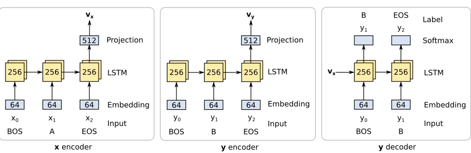
Figure 1:Neural network architectures used in our experiments. The context encoder network is used for both encoder-encoder and encoder-decoder models to encode the context sequence (‘A’) into avx. For the encoder-encoder model, label sequence (‘B’) are encoded intovyby the label encoder network. For the encoder-decoder network, the label sequence is decomposed using the chain rule by the decoder network.
efficiently in our network because the vectors vy for the sequencesyin the whitelistW can be pre-computed. Given an inputx, we computevxand take dot-product with the pre-computed vectors to find the highest scoring response. This gives us the optimal response. WhenW is very large, we can obtain an
approximate solution by indexing the vectorsvyof
W using recent methods specifically designed for dot-product based retrieval (Guo et al., 2016).
3.3 Margin
It is well-known that the maximum likelihood train-ing objective of a globally normalized model is mar-gin maximizing (Rosset et al., 2003). We illustrate this property using our set up from Claim 2.1 where a correct outputy+is of length`and an incorrect
outputy−is of length 1 with two possible labels for
each position (m= 2).
The globally conditioned model learns a parameter per possible sequence and assigns the probability to each sequence using a softmax over those parame-ters. Additionally, we place a Gaussian prior on the parameters with a precisionc. The loss for a positive
example becomes:
LG(y+) =−log
e−θy+
P y0e−θy0
+ c 2
X
y0 θ2y0,
where the sums are taken over all possible sequences.
We also train an ED model on this task. It also learns a parameter for every possible sequence, but assigns probability to each sequence using the chain rule. We also place the same Gaussian prior as above on the parameters. Letyj denote the firstj tokens
{y1, . . . , yj}of sequencey. The loss for a positive example for this model is then:
LL(y+) =− ` X
j=1
log e
−θy+
j P
y0
je
−θy0
j
+ c 2
X
y0
j θ2y0
j ,
where the inner sums are taken over all sequences of lengthj.
We train both models on synthetic sequences gen-erated using the following rule. The first token is chosen to be ‘1’ probability 0.6. If ‘1’ is chosen, it means that this is a positive example and the remain-ing`−1tokens are chosen to be ‘1’ with probability 0.9`−11. If a ‘0’ is chosen as the first token, then that
is a negative example, and the sequence generation does not go further. This means that there are2`−1
unique positive sequences of length`and one
0.0 0.2 0.4 0.6 0.8 1.0 c
0.4 0.2 0.0 0.2 0.4
Margin
Global margin ED margin ED local margin
2 3 4 5
`
0.4 0.2 0.0 0.2 0.4
Margin
[image:6.612.79.271.71.221.2]Global margin ED margin ED local margin
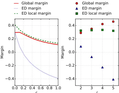
Figure 2:Comparing final margins of ED model with a glob-ally conditioned model on example dataset of Section 3.3 as a function of regularization constantcand message length`.
Adagrad (Duchi et al., 2011) for 1000 epochs with a learning rate of 0.1, effectively to convergence.
Figure 2 shows the margin for both models (be-tween the most likely correct sequence and the incor-rect sequence) and the local margin for the ED model at the end of training. On the left panel, we used sequences with`= 2and varied the regularization
constantc. Whencis zero, both models learn the
same global margin, but as it is increased the margin for the ED model decreases and becomes negative atc >0.2, despite the local margin remaining
pos-itive and high. On the right panel we usedc = 0.1
and varied`. The ED model becomes unable to
sep-arate the sequences with length above 2 with this regularization constant setting.
4 Experiments
4.1 Datasets and Tasks
We contrast the quality of the ED and encoder-encoder models on two conversational datasets: Open Subtitles and Reddit Comments.
4.1.1 Open Subtitles Dataset
The Open Subtitles dataset consists of transcrip-tions of spoken dialog in movies and television shows (Lison and Tiedemann, 2016). We restrict our model-ing only to the English subtitles, of which results in
319million utternaces. Each utterance is tokenized
into word and punctuation tokens, with the start and end marked by the BOS and EOS tokens. We
ran-domly split out90%of the utterances into the training
set, placing the rest into the validation set. As the speaker information is not present in this data set, we treat each utterance as a label sequence, with the preceding utterances as context.
4.1.2 Reddit Comments Dataset
The Reddit Comments dataset is constructed from publicly available user comments on submissions on the Reddit website. Each submission is associated with a list of directed comment trees. In total, there are 41 million submissions and 501 million
com-ments. We tokenize the individual comments in the same way as we have done with the utternaces in the Open Subtitles dataset. We randomly split90%of
the submissions and the associated comments into the training set, and the rest into the validation set. We use each comment (except the ones with no par-ent commpar-ents) as a label sequence, with the context sequence composed of its ancestor comments.
4.1.3 Whitelist and Vocabulary
From each dataset, we derived a dictionary of20
thousand most commonly used tokens. Additionally, each dictionary contained the unknown token (UNK), BOS and EOS tokens. Tokens in the datasets which were not present in their associated vocabularies were replaced by the UNK token.
From each data set, we extracted10million most
common label sequences that also contained at most
100tokens. This set of sequences was used as the
negative sample pool for the encoder-encoder models. For evaluation we created a whitelistW out of the
100thousand most common sequences. We removed
any sequence from this set that contained any UNK tokens to simplify inference.
4.1.4 Sequence Prediction Task
To evaluate the quality of these models, we task them to predict the true label sequence given its context. Due to the computational expense, we sub-sample the validation data sets to around1
probable predictions according to the model. For encoder-encoder models we use an exhaustive search over the evaluation set of common messages. For ED models we use a beam search with width ranging from1to15over a token prefix trie constructed from
the sequences inW.
4.2 Model Structure and Training Procedure
The context encoder, label encoder and decoder are implemented using LSTM recurrent networks (Hochreiter and Schmidhuber, 1997) with peephole connections (Sak et al., 2014). The context and label token sequences were mapped to embedding vectors using a lookup table that is trained jointly with the rest of the model parameters. The recurrent nets were unrolled in time up to100time-steps, with label
sequences of greater length discarded and context sequences of greater length truncated.
The decoder in the ED model is trained by using the true label sequence prefix as input, and a shifted label sequence as output (Sutskever et al., 2014). The partition function in the softmax over tokens is es-timated using importance sampling with a unigram distribution over tokens as the proposal distribution (Jean et al., 2014). We sample512negative examples
fromQ(y)to estimate the partition function for the
encoder-encoder model. See Figure 1 for connectiv-ity and network size details.
All models were trained using Adagrad (Duchi et al., 2011) with an initial base learning rate of0.1
which we exponentially decayed with a decade of
15million steps. For stability, we clip the L2 norm
of the gradients to a maximum magnitude of 1as
described in (Pascanu et al., 2012). All models are trained for30million steps with a mini-batch size of
64. The models are trained in a distributed manner on CPUs and NVidia GPUs using TensorFlow (Abadi et al., 2015).
4.3 Results
We first demonstrate the discrepancy between the local and global margin in the ED models as dis-cussed in Section 3.3. We used a beam size of 15 to get the top prediction from our trained ED mod-els on the test data and focussed on the subset for which the top prediction was incorrect. We measured local and global margin between the top predicted sequence (y−) and the correct test sequence (y+) as
follows: Global margin is the difference in their full sequence log probability. Local margin is the differ-ence in the local token probability of the smallest positionj wherey−j 6= yj+, that is local margin is Pr(y+j |y1+...j−1,x, θ)−Pr(yj−|y+1...j−1,x, θ). Note
the training loss of ED models directly compares only the local margin.
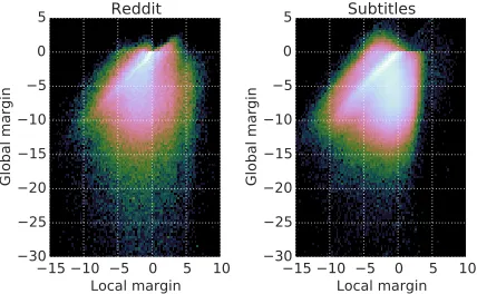
Global margin is much smaller than local margin
In Figure 3 we show the local and global margin as a 2D histogram with color luminosity denoting fre-quency. We observe that the global margin values are much smaller than the local margins. The prominent spine is for(y+,y−)pairs differing only in a single
position making the local and global margins equal. Most of the mass is below the spine. For a significant fraction of cases (27% for Reddit, and 21% for Sub-titles), the local margin is positive while the global margin is negative. That is, the ED loss for these sequences is small even though the log-probability of the correct sequence is much smaller than the log-probability of the predicted wrong sequence.
Beam search is not the bottleneck An interesting side observation from the plots in Figure 3 is that more than 98% of the wrong predictions have a nega-tive margin, that is, the score of the correct sequence is indeed lower than the score of the wrong predic-tion. Improving the beam-width beyond 15 is not likely to improve these models since only in 1.9% and 1.7% of the cases is the correct score higher than the score of the wrong prediction.
15 10 5 0 5 10 Local margin 30
25 20 15 10 5 0 5
Global margin
15 10 5 0 5 10 Local margin 30
25 20 15 10 5 0 5
Global margin
[image:7.612.316.530.512.644.2]Subtitles
Margin discrepancy is higher for longer se-quences In Figure 4 we show that this discrep-ancy is significantly more pronounced for longer sequences. In the figure we show the fraction of wrongly predicted sequences with a positive local margin. We find that as sequence length increases, we have more cases where the local margin is posi-tive yet the global margin is negaposi-tive. For example, for the Reddit dataset half of the wrongly predicted sequences have a positive local margin indicating that the training loss was low for these sequences even though they were not adequately separated.
0 1 2 3 4 5 6 7 8 >8 0
0.15 0.3 0.45 0.6
Sequence Length
Subtitles
0 1 2 3 4 5 6 7 8 >8 0
0.1 0.2 0.3 0.4
[image:8.612.315.499.60.289.2]Sequence Length
Figure 4:Fraction of incorrect predictions with positive local margin.
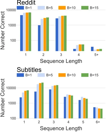
Increasing beam size drops accuracy for long se-quences Next we show why this discrepancy leads to non-monotonic accuracies with increasing beam-size. As beam size increases, the predicted se-quence has higher probability and the accuracy is expected to increase if the trained probabilities are well-calibrated. In Figure 5 we plot the number of correct predictions (on a log scale) against the length of the correct sequence for beam sizes of 1, 5, 10, and 15. For small sequence lengths, we indeed ob-serve that increasing the beam size produces more accurate results. For longer sequences (length>4) we observe a drop in accuracy with increasing the beam width beyond 1 for Reddit and beyond 5 for Subtitles.
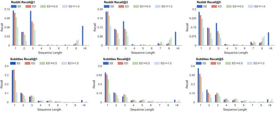
Globally conditioned models are more accurate than ED models We next compare the ED model with our globally conditioned encoder-encoder (EE) model. In Figure 6 we show the recall@K values for K=1, 3 and 5 for the two datasets for increasing length of correct sequence. We find the EE model is largely better that the ED model. The most in-teresting difference is that for sequences of length greater than 8, the ED model has a recall@5 of zero for both datasets. In contrast, the EE model manages
B=1 B=5 B=10 B=15
1 2 3 4 5+
100 1000 10000
Sequence Length
Number Correct
Subtitles
B=1 B=5 B=10 B=15
1 2 3 4 5 6+
100 1000 10000
Sequence Length
Number Correct
Figure 5:Effect of beam width on the number of correct predic-tions broken down by sequence length.
to achieve significant recall even at large sequence lengths.
Length normalization of ED models A common modification to the ED decoding procedure used to promote longer message is normalization of the pre-diction log-probability by its length raised to some powerf (Cho et al., 2014; Graves, 2013). We
ex-perimented with two settings,f = 0.5and1.0. Our
experiments show that while this indeed promotes longer sequences, it does so at the expense of reduc-ing the accuracy on the shorter sequences.
5 Related Work
In this paper we showed that encoder-decoder mod-els suffer from length bias and proposed a fix us-ing global conditionus-ing. Global conditionus-ing has been proposed for other RNN-based sequence pre-diction tasks in (Yao et al., 2014) and (Andor et al., 2016). The RNN models that these work attempt to fix capture only a weak form of dependency among variables, for example they assumexis seen
incre-mentally and only adjacent labels inyare directly
[image:8.612.72.291.234.303.2]Reddit Recall@1
EE ED ED f=0.5 ED f=1.0
1 2 3 4 5 6 7 8 >8
0 0.03 0.06 0.09 0.12
Sequence Length
Recall
Reddit Recall@3
EE ED ED f=0.5 ED f=1.0
1 2 3 4 5 6 7 8 >8
0 0.06 0.12 0.18 0.24
Sequence Length
Recall
Reddit Recall@5
EE ED ED f=0.5 ED f=1.0
1 2 3 4 5 6 7 8 >8
0 0.075 0.15 0.225 0.3
Sequence Length
Recall
Subtitles Recall@1
EE ED ED f=0.5 ED f=1.0
1 2 3 4 5 6 7 8 >8
0 0.1 0.2 0.3 0.4
Sequence Length
Recall
Subtitles Recall@3
EE ED ED f=0.5 ED f=1.0
1 2 3 4 5 6 7 8 >8
0 0.15 0.3 0.45 0.6
Sequence Length
Recall
Subtitles Recall@5
EE ED ED f=0.5 ED f=1.0
1 2 3 4 5 6 7 8 >8
0 0.15 0.3 0.45 0.6
Sequence Length
[image:9.612.80.533.59.245.2]Recall
Figure 6:Comparing recall@1, 3, 5 for increasing length of correct sequence.
global conditioning will compromise a ED model which does not assumeany conditional independence
among variables. The label-bias proof of (2016) is not applicable to ED models because the proof rests on the entire input not being visible during output. Earlier illustrations of label bias of MeMMs in (Bot-tou, 1991; Lafferty et al., 2001) also require local observations. In contrast, the ED model transitions on the entire input and chain rule is an exact factoriza-tion of the distribufactoriza-tion. Indeed one of the suggesfactoriza-tions in (Bottou, 1991) to surmount label-bias is to use a fully connected network, which the ED model al-ready does.
Our encoder-encoder network is reminiscent of the dual encoder network in (Lowe et al., 2015), also used for conversational response generation. A cru-cial difference is our use of importance sampling to correctly estimate the probability of a large set of candidate responses, which allows us to use the model as a standalone response generation system. Other differences include our model using separate sets of parameters for the two encoders, to reflect the assymetry of the prediction task. Lastly, we found it crucial for the model’s quality to use multiple appro-priately weighed negative examples for every positive example during training.
(Ranzato et al., 2016) also highlights limitations of the ED model and proposes to mix the ED loss with a sequence-level loss in a reinforcement learning framework under a carefully tuned schedule. Our method for global conditioning can capture
sequence-level losses like BLEU score more easily, but may also benefit from a similar mixed loss function.
6 Conclusion
We have shown that encoder-decoder models in the regime of finite data and parameters suffer from a length-bias problem. We have proved that this arises due to the locally normalized models insufficiently separating correct sequences from incorrect ones, and have verified this empirically. We explained why this leads to the curious phenomenon of decreasing accu-racy with increasing beam size for long sequences. Our proposed encoder-encoder architecture side steps this issue by operating in sequence probability space directly, yielding improved accuracy for longer se-quences.
One weakness of our proposed architecture is that it cannot generate responses directly. An interesting future work is to explore if the ED model can be used to generate a candidate set of responses which are then re-ranked by our globally conditioned model. Another future area is to see if the techniques for making Bayesian networks discriminative can fix the length bias of encoder decoder networks (Peharz et al., 2013; Guo et al., 2012).
References
Large-scale machine learning on heterogeneous sys-tems. Software available from tensorflow.org.
[Abadie et al.2014] J Pouget Abadie, D Bahdanau, B van Merrienboer, K Cho, and Y Bengio. 2014. Over-coming the curse of sentence length for neural ma-chine translation using automatic segmentation. CoRR, abs/1409.1257.
[Andor et al.2016] D Andor, C Alberti, D Weis, A Severyn, A Presta, K Ganchev, S Petrov, and M Collins. 2016. Globally normalized transition-based neural network.
CoRR, abs/1603.06042.
[Bahdanau et al.2014] Dzmitry Bahdanau, Kyunghyun Cho, and Yoshua Bengio. 2014. Neural machine trans-lation by jointly learning to align and translate. CoRR, abs/1409.0473.
[Bengio et al.2015] Samy Bengio, Oriol Vinyals, Navdeep Jaitly, and Noam Shazeer. 2015. Scheduled sampling for sequence prediction with recurrent neural networks. InNIPS.
[Bottou1991] L. Bottou. 1991. Une approche theorique de l’apprentissage connexionniste: Applications a la re-con‘naissance de la parole. Ph.D. thesis, Universitede Paris XI.
[Cho et al.2014] KyungHyun Cho, Bart van Merrienboer, Dzmitry Bahdanau, and Yoshua Bengio. 2014. On the properties of neural machine translation: Encoder-decoder approaches. CoRR, abs/1409.1259.
[Duchi et al.2011] John Duchi, Elan Hazad, and Yoram Singer. 2011. Adaptive subgradient methods for online learning and stochastic optimization. JMLR, 12. [Graves2013] Alex Graves. 2013. Generating sequences
with recurrent neural networks.CoRR, abs/1308.0850. [Guo et al.2012] Yuhong Guo, Dana F. Wilkinson, and Dale Schuurmans. 2012. Maximum margin bayesian networks. CoRR, abs/1207.1382.
[Guo et al.2016] R. Guo, S. Kumar, K. Choromanski, and D. Simcha. 2016. Quantization based fast inner prod-uct search. InAISTATS.
[Hochreiter and Schmidhuber1997] Sepp Hochreiter and Jürgen Schmidhuber. 1997. Long short-term memory.
Neural computation, 9(8):1735–1780.
[Jean et al.2014] Sébastien Jean, Kyunghyun Cho, Roland Memisevic, and Yoshua Bengio. 2014. On using very large target vocabulary for neural machine translation.
CoRR, abs/1412.2007.
[Kannan et al.2016] Anjuli Kannan, Karol Kurach, Sujith Ravi, Tobias Kaufmann, Andrew Tomkins, Balint Mik-los, Greg Corrado, László Lukács, Marina Ganea, Peter Young, and Vivek Ramavajjala. 2016. Smart reply: Automated response suggestion for email. InKDD.
[Khaitan2016] Pranav Khaitan.
2016. Chat smarter with allo.
http://googleresearch.blogspot.com/2016/05/chat-smarter-with-allo.html, May.
[Lafferty et al.2001] John Lafferty, Andrew McCallum, and Fernando Pereira. 2001. Conditional random fields: Probabilistic models for segmenting and labeling sequence data. InICML.
[Li et al.2015] J Li, M Galley, C Brockett, J Gao, and B Dolan. 2015. A diversity-promoting objective function for neural conversation models. CoRR, abs/1510.03055.
[Lison and Tiedemann2016] Pierre Lison and Jörg Tiede-mann. 2016. Opensubtitles2016: Extracting large parallel corpora from movie and tv subtitles. InLREC 2016.
[Lowe et al.2015] R Lowe, N Pow, I V Serban, and J Pineau. 2015. The ubuntu dialogue corpus: A large dataset for research in unstructure multi-turn dialogue systems". InSIGDial.
[McCallum et al.2000] A. McCallum, D. Freitag, and F. Pereira. 2000. Maximum entropy markov mod-els for information extraction and segmentation. In
ICML.
[Pascanu et al.2012] Razvan Pascanu, Tomas Mikolov, and Yoshua Bengio. 2012. Understanding the explod-ing gradient problem. CoRR, abs/1211.5063.
[Peharz et al.2013] Robert Peharz, Sebastian Tschiatschek, and Franz Pernkopf. 2013. The most generative maxi-mum margin bayesian networks. InICML.
[Ranzato et al.2016] M Ranzato, S Chopra, M Auli, and W Zaremba. 2016. Sequence level training with recur-rent neural networks. ICLR.
[Rosset et al.2003] S Rosset, J Zhu, and T Hastie. 2003. Margin maximizing loss functions. InNIPS.
[Sak et al.2014] Hasim Sak, Andrew Senior, and Francoise Beaufays. 2014. Long Short-Term Memory Recurrent Neural Network Architectures for Large Scale Acoustic Modeling. InINTERSPEECH 2014.
[Sutskever et al.2014] Ilya Sutskever, Oriol Vinyals, and Quoc V. Le. 2014. Sequence to sequence learning with neural networks. InNIPS.
[Vinyals and Le2015] Oriol Vinyals and Quoc V. Le. 2015. A neural conversational model. CoRR, abs/1506.05869.
[Vinyals et al.2015] Oriol Vinyals, Alexander Toshev, Samy Bengio, and Dumitru Erhan. 2015. Show and tell: A neural image caption generator. InCVPR. [Yao et al.2014] K Yao, B Peng, G Zweig, D Yu, X Li, and