The Hamiltonian Cycle Problem on Circular-Arc Graphs
∗
Ruo-Wei Hung
†‡, Maw-Shang Chang
§, and Chi-Hyi Laio
Abstract—A Hamiltonian cycle in a graph G is a simple cycle in which each vertex of G appears ex-actly once. The Hamiltonian cycle problem involves testing whether a Hamiltonian cycle exists in a graph, and finds one if such a cycle does exist. It is well known that the Hamiltonian cycle problem is one of the classic NP-complete problems on general graphs. Shih et al. solved the Hamiltonian cycle problem on circular-arc graphs in O(n2logn)time [36], where n is the number of vertices of the input graph. Whether there exists a more efficient algorithm for solving the Hamiltonian cycle problem on circular-arc graphs has been opened for a decade. In this paper, we present anO(∆n)-time algorithm to solve it, where∆denotes the maximum degree of the input graph.
Keywords: graph algorithms, Hamiltonian cycle prob-lem, path cover probprob-lem, interval graphs, circular-arc graphs
1
Introduction
All graphs considered in this paper are finite and undi-rected, without loops or multiple edges. Let G= (V, E) be a graph with vertex set V and edge setE. Through-out this paper, let m, n, and ∆ denote the number of edges, the number of vertices, and the maximum degree of G, respectively. A Hamiltonian cycle in G is a sim-ple cycle in which each vertex ofGappears exactly once. AHamiltonian path in Gis a simple path with the same property. TheHamiltonian cycle(resp. path)problem in-volves testing whether or not Gcontains a Hamiltonian cycle (resp. path), and finds one if such a cycle (resp. path) does exist. A graphGis said to beHamiltonian if it contains a Hamiltonian cycle. TheHamiltonian prob-lemsinclude the Hamiltonian path and Hamiltonian cycle problems and have numerous applications in different ar-eas, including establishing transport routes, production launching, the on-line optimization of flexible manufac-turing systems [2], computing the perceptual boundaries of dot patterns [33], and pattern recognition [3, 34, 37]. It is well known that the Hamiltonian problems are
NP-∗The research was supported in part by the National Science
Council of Taiwan under grant no. NSC95-2221-E-324-056.
†Department of Computer Science and Information
Engineer-ing, Chaoyang University of Technology, Wufong, Taichung 413, Taiwan.
‡Corresponding author’s e-mail: [email protected]
§Department of Computer Science and Information
Engineer-ing, National Chung Cheng University, Ming-Hsiung, Chiayi 621, Taiwan.
complete for general graphs [15, 25]. The same holds true for bipartite graphs [26], split graphs [16], circle graphs [9], undirected path graphs [4] and grid graphs [24]. How-ever, polynomial time algorithms exist for the Hamilto-nian cycle or HamiltoHamilto-nian path problem on some special classes of graphs, such as interval graphs [1, 7], permuta-tion graphs [13, 35], cocomparability graphs [10, 12], and distance-hereditary graphs [17, 20, 22]. A path cover of a graph Gis a family of vertex-disjoint paths that cov-ers all vertices of G. Given a graph G, the path cover problem is to find a path cover of G of minimum num-ber, denoted byπ(G), of paths. This problem is NP-hard for general graphs [15] since it contains the Hamiltonian path problem as a special case.
A graphG= (V, E) is called anintersection graph for a finite family F of nonempty sets if there is a one-to-one correspondence between F and V such that two sets in
F have nonempty intersection if and only if their corre-sponding vertices in V are adjacent. We call F an in-tersection model of G. For an intersection modelF, we use G(F) to denote the intersection graph for F. If F is a family of intervals on a real line, thenGis called an interval graph forF andFis called aninterval model of
G. If F is a family of arcs on a circle, then G is called a circular-arc graph for F and F is called a circular-arc model of G. The two classes of interval graphs and circular-arc graphs have a variety of applications involv-ing traffic light sequencinvolv-ing, VLSI design, schedulinvolv-ing [16], and genetics [39].
Shih et al. solved the Hamiltonian cycle problem on circular-arc graphs in O(n2logn) time [36]. Whether there exists an efficient algorithm whose time-complexity is better than O(n2logn) for solving the Hamiltonian cycle problem on circular-arc graphs has been opened for a decade. In this paper, we present an O(∆n )-time algorithm to solve it. We explain our strategy by briefly describing the algorithm as follows. It reduces the problem to the Hamiltonian cycle problem and the path cover problem on interval graphs and uses anO(n )-time algorithm proposed by Chang et al. [7] for interval graphs. Note that interval graphs form a proper subclass of circular-arc graphs. The basic idea is described in the following. We first convert the circular-arc model F to an interval modelI, whereG(I) is a spanning subgraph of G(F). If G(I) is Hamiltonian, then G(F) is Hamil-tonian. If G(I) is not Hamiltonian, then a subset C of
connected components. IfG(F\C) has|C|+ 1 connected components, thenG(F) is not Hamiltonian by pigeonhole principle. Otherwise, a nonempty subsetEC of edge set ofG(F) is found. Every edgeeofEC connects two arcs ofC andG(F) is obtained by removingEC fromG(F). Furthermore, G(F) is still a circular-arc graph. By pi-geonhole principle, every edgeeofEC will not be in any Hamiltonian cycle of G(F). Thus, G(F) is Hamiltonian if and only if G(F) is Hamiltonian. Let F = F and repeat the above process until the problem is solved.
Related works are summarized below. Arikati and Ran-gan presented anO(n+m)-time algorithm to solve the path cover problem on interval graphs [1]. Chang et al. proposedO(n)-time algorithms for both the Hamiltonian cycle and path cover problems on interval graphs given an interval model that is a set of nsorted intervals [7]. Damaschke presented an O(n5)-time algorithm to solve the Hamiltonian path problem on circular-arc graphs [11]. Shih et al. proposed an O(n2logn)-time algorithm for the Hamiltonian cycle problem on circular-arc graphs [36]. The algorithm proposed by Bonuccelli and Bovet for solving the path cover problem on circular-arc graphs [5] contains a flaw which was pointed out in [36]. Some researchers [6, 28, 29] claimed thatO(n)-time algorithms exist for the Hamiltonian cycle problem and the path cover problem on circular-arc graphs given a circular-arc model that is a set ofnsorted arcs, but they have not yet succeeded in proving the correctness of their algorithms. In [23], we presented an O(n)-time approximation algo-rithm for the path cover problem on circular-arc graphs. We showed that the cardinality of the path cover found by the approximation algorithm is at most one more than the optimal one. By using the result, we reduced the path cover problem on circular-arc graphs to the Hamiltonian cycle problem on the same class of graphs inO(n) time.
The paper is organized as follows. In Section 2, we estab-lish the notation and related terminology, and review a greedy algorithm for the path cover problem on interval graphs. In Section 3, we present an O(∆n)-time algo-rithm to solve the Hamiltonian cycle problem on circular-arc graphs. Section 4 reveals how to prove the correct-ness of our algorithm, analyzes the complexity of our algorithm, and introduces a technique that reduces the related problems to the Hamiltonian cycle problem on circular-arc graphs. Finally, in Section 5 we conclude the paper and discuss possible future researches.
2
Preliminaries
In this section, we establish basic terminology and review a greedy algorithm for solving the path cover problem on interval graphs.
Let G= (V, E) be a graph without isolated vertices. A pathP inG, denoted byv1→v2→ · · · →v|P|−1→v|P|, is a sequence (v1, v2,· · ·, v|P|−1, v|P|) of vertices so that
two vertices are adjacent if and only if they are consecu-tive in the sequence. The first and last vertices visited by
P are called the path-start and path-end of P, denoted bystart(P) andend(P), respectively. We callvithe pre-decessor of vi+1, denoted by vi =predecessor(vi+1), in
P, for 1 ≤ i ≤ |P| −1. We use vi ∈ P to denote “P
visits vi”. In addition, we will use P to refer to the set of vertices visited by pathP if it is understood without ambiguity. For any S ⊆V, G\S denotes the subgraph ofGinduced byV\S, i.e.,G\S=G[V\S]. A subsetC
of vertices ofGis called acutsetif the removal ofCfrom
GdisconnectsG. We callC aconnecting set ofGifCis a cutset of G and the removal ofC from Gdisconnects
Ginto at least|C|+ 1 connected components.
For C ⊆V, let E(C) denote the set of edges of E that connect two vertices inC. The following two propositions can be easily verified by the pigeonhole principle.
Proposition 2.1. LetCbe a cutset of a connected graph
G and let g be the number of connected components in
G\C. Ifg >|C|, thenGhas no Hamiltonian cycle.
Proposition 2.2. LetCbe a cutset of a connected graph
G and let g be the number of connected components in
G\C such that g=|C|. Then,Gis Hamiltonian if and only if GC = (V, E\EC) is Hamiltonian, where EC is any nonempty subset ofE(C).
Our algorithm for the Hamiltonian cycle problem on circular-arc graphs reduces the problem to the path cover and Hamiltonian cycle problems on interval graphs. Arikati and Rangan presented an O(n+m)-time algo-rithm for the path cover problem on interval graphs [1]. Manacher et al. solved the Hamiltonian cycle problem on interval graphs in linear time [30]. These two algorithms can be implemented inO(n) time given an interval model that is a set ofnsorted intervals [7].
Now, we review the algorithm in [1] for the path cover problem on interval graphs. The algorithm is assumed that the input graph is given by an interval modelIthat is a set of nsorted intervals labeled by 1,2,· · · , nin in-creasing order of their right endpoints. Notice that we do not distinguish an interval from its label. The left endpoint of intervalxis denoted byleft(x) and the right endpoint by right(x). Interval xis denoted by (left(x), right(x)). An intervalxis said tocontain another inter-valyif every point ofyfalls within the interior of (left(x), right(x)). For convenience, we need the following nota-tion: (1) For two distinct intervalsx, y in I,xis smaller than y, denoted by x < y, if right(y) is to the right of right(x), and (2) s(I) denotes the interval inI with the leftmost right endpoint, i.e.,s(I)≤xforx∈I.
i1
i2
i3 i4
i5 i6 i7 i8 i9 i10
[image:3.595.49.290.71.116.2]i11 i12
Fig. 1: An interval modelI of twelve sorted intervals.
subset C of a setI of sorted intervals so that G(I\C) has at least|C|+ 1 connected components.
The algorithm presented in [1] for the path cover problem on an interval modelIuses a greedy principle to extend a
pathZi=z1→z2→ · · · →zk,k≥1. Initially,i= 1 and
Z1 visitss(I), i.e.,start(Z1) =s(I). Then, the unvisited neighbor ofzk with the leftmost right endpoint is chosen andZiis extended to visit it. If such a neighbor does not exist, thenZiis stopped and a new pathZi+1is started in the remaining graph from the smallest labeled unvisited interval if it is possible. To simplify the notation, we denote the algorithm and its output by Algorithm GP and GP(I), respectively. For instance, given a set of sorted intervals shown in Fig. 1, Algorithm GP outputs two paths Z1 = i1 → i2 → i3 → i4 → i6 → i5 and
Z2 = i7 → i8 → i9 → i10 → i12 → i11. The following theorem was given by Arikati et al. in [1] and shows the optimality of Algorithm GP.
Theorem 2.3. (Arikati et al. [1]; Hung et al. [23])
GP(I)is a minimum path cover of G(I).
It is easy to see that Algorithm GP runs in O(n+m) time. Chang et al. showed that Algorithm GP can be done inO(n) time and O(n) space given a set of sorted intervals [7]. The paths inGP(I) are calledgreedy paths. Note that the path-start of a greedy path is the smallest labeled interval in the path. Define L(Z) of a pathZ to be the collection of intervals in Z which are larger than
end(Z), i.e.,L(Z) ={x|x∈Z andend(Z)< x}. A path
Z is called a monotone path if and only ifL(Z) =∅. For instance, let Z1 =i1 → i2 → i3 → i4 → i6 → i5 be a path ofG(I) shown in Fig. 1, thenL(Z1) ={i6}. Given a greedy pathZ, we can find a subsetC(Z) ofZ so that the removal ofC(Z) fromZdisconnectsZinto|C(Z)|+1 subpaths. The procedure was given in [23]. For readers’ convenience, we describe it as follows.
Procedure GCS
Input: Z, a greedy path inGP(I).
Output: C(Z), thegreedy connecting set of pathZ, and
R(Z), the set of all of the sub-paths of Z obtained by removingC(Z) fromZ.
Method:
1. S=Z;C(Z) =∅;R(Z) =∅;
2. z=end(Z);CurrentP athEnd=end(Z); 3. whilez=start(S)do
4. letz=predecessor(z);
5. if CurrentP athEnd < z,then
6. letS=S1→z→S2, whereS1 andS2 are two subpaths ofS;
7. C(Z) =C(Z)∪ {z};R(Z) =R(Z)∪ {S2}; 8. S=S1;z=CurrentP athEnd=end(S1); 9. R(Z) =R(Z)∪ {S};
10. outputC(Z) andR(Z).
For instance, given a greedy pathZ1 =i1→i2 →i3→ i4→i6→i5of Fig. 1, Procedure GCS outputsC(Z1) =
{i6} and R(Z1) = {i1 → i2 → i3 → i4, i5}. Since each interval is visited once, Procedure GCS(Z) runs inO(|Z|) time.
3
The Hamiltonian Cycle Algorithm
Circular-arc graphs are simple generalization of interval graphs. However, circular-arc graphs have rich structure, and there is a long history for the recognition problem. Tucker presented an O(n3)-time algorithm for testing whether a graph is a circular-arc graph [38]. Hsu pro-posed anO(mn)-time algorithm to recognize circular-arc graphs [19]. Eschen and Spinrad proposed an O(n2 )-time recognition algorithm for circular-arc graphs [14]. Now, an O(m+n)-linear-time recognition algorithm for circular-arc graphs has been proposed by McConnell in [32]. A circular-arc model F can be obtained by these recognition algorithms in the affirmative case. Hence, researchers studying circular-arc graphs sometimes as-sumed that a set of arcs with endpoints sorted is given [7, 8, 18, 21, 31]. In the following, we assume that the input graph is given by a circular-arc modelF that is a set of nsorted arcs.
An arc xin F that begins with endpointpand ends at endpointqin clockwise direction is denoted by (p, q). We call pthehead, denoted byh(x), andq thetail, denoted by t(x), of arc (p, q). The contiguous part of the circle that begins with an endpointc and ends at an endpoint
d in clockwise direction is referred to as segment (c, d), denoted by seg(c, d), of the circle. We use “arc” to refer to a member ofF and “segment” to refer to a part of the circle between two endpoints. A point y on the circle is said to be contained in arc (or segment) (p, q) if it falls within the interior of seg(p, q). An arc or segment xis said to contain another arc or segment y if x contains every point of y. Two arcs, or two segments, or an arc and a segmentintersect if and only if they share a point. For a pointqon the circle, letBp(q) be the set of all arcs in F containing point q. For an arc x in F, let Ba(x) be the set of all arcs in F containing arc x. Without loss of generality, we assume that (1) all endpoints are distinct, (2) no arc covers the entire circle, and (3) an arc (segment) does not include its two endpoints, i.e., it is an open segment of the circle.
cir-cle from the head (resp. tail) of an arc v and stretches the circle into a horizontal line. Thus an arc becomes an interval. We stretch the circle in this way such that the head (resp. tail) of arc v is on the left hand side of the horizontal line. In other words,h(v) (resp. t(v)) becomes the left endpoint of the corresponding interval of arc v. An arc that contains the cut point is not cut into two in-tervals but is stretched into an interval. LetBbe a subset of Ba(v). Note that Bis a part of the input of this pro-cedure. Those arcs inB are stretched into intervals that contain the left endpoint of the corresponding interval of arcv. Those arcs that contain the cut point but are not in B are stretched into intervals that do not contain the left endpoint of the corresponding interval of arc v. The mapping procedure that cuts the circle from h(v) (resp.
t(v)) is calledclockwise(resp. counterclockwise) mapping with respect to arc vand Band is formally presented as follows.
Procedure ArcToI
Input: A set F of n sorted arcs, an arc v ∈ F, and a subsetBofBa(v).
Output: A set Ic(B, v) (resp. Icc(B, v)) of nsorted in-tervals.
Method:
1. starting from pointh(v) (resp. t(v)), label the end-points of arcs ofF in clockwise (resp. counterclock-wise) direction; that is, the endpoint located on point
h(v) (resp. t(v)) is labeled by 1; 2. let(p) denote the label of endpointp;
3. for each arc x ∈ B, x is mapped to interval
Ic(x) = (h(x), t(x)) if (t(x)) > (h(x)) (resp.
Icc(x) = (t(x), h(x)) if (h(x)) > (t(x))) and to interval Ic(x) = (h(x), t(x) + 2n) (resp. Icc(x) = (t(x), h(x) + 2n)) otherwise;
4. foreach arcx∈ B,xis mapped to intervalIc(x) = (1, t(x)) (resp. Icc(x) = (1, h(x)));
5. let Ic(B, v) = {Ic(x)|x ∈ F} (resp. Icc(B, v) =
{Icc(x)|x ∈ F}) and output Ic(B, v) (resp.
Icc(B, v)).
Apparently, both G(Ic(B, v)) and G(Icc(B, v)) are span-ning subgraphs of G(F). For instance, given a set F of arcs shown in Fig. 2, arca1, andB=Ba(a1), Procedure ArcToI first labels the endpoints of arcs ofF (as shown in Fig. 3) in clockwise direction starting fromh(a1). Then, it converts F into a set Ic(Ba(a1), a1)) of intervals as shown in Fig. 4. On the other hand, Procedure ArcToI constructs a setIcc(∅, a6) (as shown in Fig. 5) of intervals for the setF of arcs shown in Fig. 2. Careful implemen-tation of Procedure ArcToI takes O(n) time and O(n) space.
Letvbe an arc in a setF of arcs,Bbe a subset ofBa(v),
Ic and Icc representIc(B, v) and Icc(B, v), respectively, and letIbe eitherIc orIcc. Letxbe an arc inF and let
a1 a2
a3
a4
a5
a6
a7
a8
a9
[image:4.595.352.503.71.231.2]a10 a11
Fig. 2: A circular-arc modelF of eleven sorted arcs.
a1 a2
a3
a4
a5
a6
a7
a8
a9
a10
a11 1
2
3 4 5
6 7
8 9 11 12 13
15 16 17 1819
20 21
10
[image:4.595.350.503.284.443.2]14 22
Fig. 3: The clockwise labeling by Procedure ArcToI given
F shown in Fig. 2, arca1, andB=Ba(a1), where dashed lines indicate the removed segments of arcs fromF.
X be a subset of F. We use I(x) to denote the interval corresponding to arcxinIandI(X) to denote{I(x)|x∈ X}. Conversely, lety be an interval in I and letY be a subset ofI. We useF(y) to denote the arc corresponding toy in F andF(Y) to denote{F(y)|y∈Y}.
Now, we present an O(∆n)-time algorithm to solve the Hamiltonian cycle problem on circular-arc graphs. Our algorithm reduces the problem to the Hamiltonian cycle and the path cover problems on interval graphs. Note that the Hamiltonian cycle and the path cover problems on interval graphs can be solved inO(n) time if the input is a set ofnintervals with endpoints sorted [1, 7, 30]. The algorithm is formally presented as follows.
Algorithm HC(F)
Input: F, a set of sorted arcs.
Output: A Hamiltonian cycle ofG(F) if it is Hamilto-nian.
a1 a3 a4
a2
a5
a6
a7 a8
a9
a10
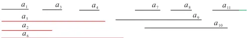
[image:5.595.46.294.70.109.2]a11
Fig. 4: The setIc(Ba(a1), a1) of intervals for the setF of arcs shown in Fig. 2.
a1 a3
a4
a2 a5
a6 a8 a7
[image:5.595.46.290.166.208.2]a9 a10 a11
Fig. 5: The setIcc(∅, a6) of intervals for the setF of arcs shown in Fig. 2.
Step 1: Map F into a set Ic of intervals in a clockwise direction and test whetherG(Ic) is Hamiltonian. (1.1) pick an arc µ of F that does not contain any other arc;
(1.2) map F into a set Ic = Ic(Ba(µ), µ) of inter-vals by calling Procedure ArcToI that is a clockwise mapping w.r.t. Ba(µ) andµ;
(1.3) call Algorithm GP to computeGP(Ic); (1.4) let P be the first greedy path output by Algo-rithm GP(Ic) and letυ be the arc corresponding to
end(P);
(1.5) if |GP(Ic)| = 1 and arcµ intersects arc υ in
G(F),then output “υ→P” as a Hamiltonian cy-cle of G(F) andterminatethe algorithm.
(1.6) if G(Ic) is Hamiltonian, then output the Hamiltonian cycle found in G(Ic) and terminate
the algorithm. /* call the algorithm in [7, 30] to test whetherG(Ic) is Hamiltonian or not */
Step 2: Map F into a set Icc of intervals in a counter-clockwise direction and computeGP(Icc).
(2.1) call Procedure GCS(P) to findL(P) andC(P), where P = P1 →c1 →P2 → · · · →ck−1 → Pk → ck→Pk+1 andC(P) ={c1, c2,· · · , ck};
(2.2) letυ1 be the arc corresponding toend(P1); (2.3) mapF into a setIcc=Icc(∅, υ1) of intervals by calling Procedure ArcToI that is a counterclockwise mapping w.r.t. ∅ andυ1;
(2.4) call Algorithm GP to computeGP(Icc);
Step 3: Test whether G(Icc) is Hamiltonian.
(3.1)if |GP(Icc)|>1,then output“G(F) has no Hamiltonian cycle” and terminatethe algorithm. (3.2) letQbe the only greedy path inGP(Icc); (3.3) let s and ω be the arcs corresponding to
start(Q) andend(Q), respectively;
(3.4) if arc s intersects arc ω in G(F), then out-put “ω → Q” as a Hamiltonian cycle ofG(F) and
terminatethe algorithm.
(3.5) if G(Icc) is Hamiltonian, then output the Hamiltonian cycle found in G(Icc) and terminate
the algorithm. /* call the algorithm in [7, 30] to test whetherG(Icc) is Hamiltonian or not */
(3.6) call Procedure GCS(Q) to findL(Q) andC(Q), where Q=Q1→d1→Q2→ · · · →dh−1 →Qh→
dh→Qh+1and C(Q) ={d1, d2,· · · , dh};
Step 4: Process the case that |GP(Icc)|= 1, arcsdoes not intersect arcω, ands=υ1.
(4.1)if ω∈Bp(t(υ1)),then gotoStep 5; (4.2) letR={r∈F|r∈Bp(h(ω))\F(L(Q))}; (4.3) let z be an arc of Rsuch that right(Icc(z)) is the smallest inIcc(R);
(4.4)if |GP(Icc\ {Icc(z)})|= 1,then
(4.5) letGP(Icc\ {Icc(z)}) ={Qz¯} and letω¯z=
F(end(Qz¯));
(4.6) if arcz intersects arcωz¯,then output
“z→Q¯z→z” as a Hamiltonian cycle of
G(F) andterminate the algorithm.
(4.7) let F = (F\ {z})∪seg(h(z), h(ω)); /* remove
seg(h(ω), t(z)) of arczfrom F */ (4.8)gotoStep 4.1;
Step 5: output “G(F) has no Hamiltonian cycle” and
terminatethe algorithm.
In the following, we give an example to explain Algorithm HC(F). LetF be the set of arcs shown in Fig. 2. The algorithm picks arc µ = a1 that does not contain any other arc. It first mapsF into the setIc of intervals by a clockwise mapping w.r.t. Ba(a1) anda1 (as shown in Fig. 4). This first greedy path P output by Algorithm GP(Ic) isa1→a2→a3→a5→a4→a6 →a9→a7→ a10→a8which is not a Hamiltonian path ofG(Ic). It is straightforward to verify that υ=F(end(P)) = a8. We find thatG(Ic) is not Hamiltonian. Next, the algorithm computesC(P) =L(P) ={a9, a10}. It is straightforward to verify thatP1=a1→a2 →a3 →a5 →a4 →a6 and
υ1=F(end(P1)) =a6. The algorithm then mapsF into the set Icc of intervals by a counterclockwise mapping w.r.t. ∅andυ1=a6 (as shown in Fig. 5). By Algorithm GP, we find that |GP(Icc)| = 1. Let GP(Icc) = {Q}. Then, Q =a4 →a6 → a3 → a5 →a1 → a11 →a10 → a8 → a9 → a7 → a2. Arc a4 = F(start(Q)) does not intersect arc a2=F(end(Q)). By the Hamiltonian cycle algorithm for interval graphs, we find that G(Icc) has a Hamiltonian cycle a4 →a6 →a3 → a2 →a1 →a11 → a10→a8→a9→a7→a5→a4. It is also a Hamiltonian cycle ofG(F).
4
Analysis of Algorithm
We first show how to prove the correctness of Algorithm HC given a set F of sorted arcs. Consider the case of
µ = υ. In this case, G(F) and G(Icc) are isomorphic [23]. Hence,G(F) is an interval graph and the algorithm is easily verified to be correct. Consider that µ = υ. Suppose µ ∈ Bp(t(υ)). In [23], we showed that P is a Hamiltonian path ofG(Ic). Hence, “υ→P” is a Hamil-tonian cycle of G(F) and the algorithm terminates at Step 1.5. Thus, Algorithm HC(F) is correct whenµ=υ
and µ∈Bp(t(υ)). From now on, we assume thatµ=υ
no arc in F covers the entire circle, and arc µ does not contain any other arc ofF.
Apparently, Algorithm HC(F) is correct if it terminates at either Step 1.5, Step 1.6, Step 3.4 or Step 3.5 since
G(Ic) and G(Icc) are spanning subgraphs of G(F). We observe that υ1 = υ if L(P) = ∅, and υ1 ∈ Ba(s) if
s=υ1. To verify the correctness of Step 4.6, we show that arczintersects bothF(start(Qz¯)) andF(end(Qz¯)), and, hence, “z→Qz¯→z” is a Hamiltonian cycle ofG(F). To verify the correctness of Steps 3.1 and 5, we find a subset
C ofF such thatG(F\ C) has at least|C|+ 1 connected components. By Proposition 2.1, G(F) is not Hamilto-nian. In Step 4.7, we remove the segmentseg(h(ω), t(z)) of arc z from F. We prove its correctness by finding a subset C of F such that z ∈ C, G(F \ C) has at least
|C|connected components, and no arcs ofF\ C intersect
seg(h(ω), t(z)). By Proposition 2.2, G(F) is Hamilto-nian if and only if graphG((F\ {z})∪seg(h(z), h(ω))) is Hamiltonian. To verify the correctness of the algorithm, we may prove the following claims. Due to the space limitation, we omit the proofs of these claims.
(1) G(F) is not Hamiltonian if|GP(Icc)|>1 (Step 3.1);
(2) G(F) is not Hamiltonian if |GP(Icc)| = 1 and ω ∈ Bp(t(υ1)) (Step 5);
(3) Suppose thatω ∈Bp(t(υ1)) (it implies R =∅) and
|GP(Icc\{Icc(z)})|= 1. Then,G(F) is Hamiltonian if and only if arc z intersects arc ωz¯in G(F) (Step 4.6);
(4) Suppose that ω ∈ Bp(t(υ1)) and |GP(Icc \
{Icc(z)})| = 1. If arcs z and ωz¯ do not intersect, thenG(F) is Hamiltonian if and only ifG((F\{z})∪
seg(h(z), h(ω))) is Hamiltonian (Step 4.7).
(5) Suppose that ω ∈ Bp(t(υ1)) and |GP(Icc \
{Icc(z)})| > 1. Then, G(F) is Hamiltonian if and only ifG((F\ {z})∪seg(h(z), h(ω))) is Hamiltonian (Step 4.7).
Next, we analyze the complexity of Algorithm HC. The algorithm is assumed that the input graph is given by a circular-arc modelF that is a set ofnsorted arcs. Given such a modelF, an arcµofF that does not contain any other arc can be easily found in O(n) time. From now on, we assume that such an arc µis given.
Manacher et al. proposed a Hamiltonian cycle algorithm on interval graphs [30]. Chang et al. implemented the algorithm in O(n) time if a set of n sorted intervals is given [7]. Hence, testing whether G(Ic) orG(Icc) has a Hamiltonian cycle can be done inO(n) time. It is easy to see that the algorithm runs inO(n) time if it terminates at either Step 1.5, Step 3.1 or Step 3.4. Therefore, the time complexity of Algorithm HC isO(n) if it terminates before Step 4. Consider that Algorithm HC does not terminate before Step 4. Let ∆ω be the number of arcs in Bp(h(ω)). Clearly, ∆ω ≤ ∆. Let R = {r ∈ F|r ∈
Bp(h(ω))\F(L(Q))}. In each iteration of Step 4, |R|is decreased by 1. Obviously,|R| ≤∆ω. Therefore, Step 4 is iterated at most|R|times, and, hence, it is iterated at most ∆ω times. Since every line can be implemented in
O(n) time, Step 4 runs inO(∆n) time. Thus, we conclude the following theorem.
Theorem 4.1. Given a circular-arc modelFthat is a set of n sorted arcs, Algorithm HC solves the Hamiltonian cycle problem on G(F)inO(∆n)time.
In [23], we proposed an O(n)-time approximation al-gorithm for the path cover problem on a circular-arc graph G(F). Let π be the cardinality of the path cover found by the approximation algorithm. We showed that
π ≤π(G(F)) + 1 in [23]. Then, the path cover problem onG(F) can be solved by reducing it to the Hamiltonian cycle problem as follows. Ifπ = 1, thenπ(G(F)) = π. Otherwise,π(G(F)) =π−1 if and only ifG(F)⊗Kπ−1
is Hamiltonian, whereKπ−1is a complete graph ofπ−1 vertices,G(F) andKπ−1are disjoint, andG(F)⊗Kπ−1
is the graph obtained by connecting every vertex ofG(F) with all vertices ofKπ−1. Apparently,G(F)⊗Kπ−1 is
a circular-arc graph, too. Let ∆ be the maximum degree of G(F). Then, the maximum degree of G(F)⊗Kπ−1
is ∆ + (π−1). By using the above reduction and the Hamiltonian cycle algorithm proposed in the paper, the path cover problem onG(F) can be solved inO(n2) time. Thus, we have the following corollary.
Corollary 4.2. Given a circular-arc model F that is a set of nsorted arcs, the path cover problem onG(F)can be solved inO(n2)time.
It is well known that the Hamiltonian cycle and Hamilto-nian path problems on circular-arc graphs can be reduced to each other [23, 27]. Thus, the Hamiltonian path prob-lem on circular-arc graphs can be solved by an algorithm whose time complexity is the same as that of the most efficient algorithm for the Hamiltonian cycle problem on the same class of graphs. Therefore, the following corol-lary immediately holds true.
Corollary 4.3. Given a circular-arc model F that is a set of n sorted arcs, the Hamiltonian path problem on
G(F) can be solved inO(∆n)time.
5
Concluding Remarks
In this paper, we solve the Hamiltonian cycle problem on circular-arc graphs inO(∆n) time. This improves the best previous result in [36] for this problem which is an
paper, the path cover problem on circular-arc graphs can be solved in O(n2) time. In addition, given a circular-arc modelF that is a set ofnarcs with endpoints sorted, whether the Hamiltonian cycle or Hamiltonian path prob-lem onG(F) can be solved inO(n) time remains open.
References
[1] S.R. Arikati and C. Pandu Rangan, Linear algorithm for optimal path cover problem on interval graphs, Inform. Process. Lett.35 (1990) 149–153.
[2] N. Ascheuer, Hamiltonian path problems in the on-line optimization of flexible manufacturing systems, Technique Report TR 96-3, Konrad-Zuse-Zentrum f¨ur Informationstechnik, Berlin, 1996.
[3] J.C. Bermond, Hamiltonian graphs, in Selected Top-ics in Graph Theory ed. by L.W. Beinke and R.J. Wilson, Academic Press, New York, 1978.
[4] A.A. Bertossi and M.A. Bonuccelli, Hamiltonian cir-cuits in interval graph generalizations,Inform. Pro-cess. Lett.23(1986) 195–200.
[5] M.A. Bonuccelli and D.P. Bovet, Minimum node dis-joint path covering for circular-arc graphs, Inform. Process. Lett.8(1979) 159–161.
[6] M.S. Chang, S.L. Peng and J.L. Liaw, Deferred-query – an efficient approach for some problems on interval and circular-arc graphs, Lecture Notes in Comput. Sci., vol. 709, Springer, Berlin, 1993, pp. 222–233.
[7] M.S. Chang, S.L. Peng and J.L. Liaw, Deferred-query: an efficient approach for some problems on interval graphs,Networks 34 (1999) 1–10.
[8] D.Z. Chen, D.T. Lee, R. Sridhar and C.N. Sekharan, Solving the all-pair shortest path query problem on interval and circular-arc graphs,Networks31(1998) 249–258.
[9] P. Damaschke, The Hamiltonian circuit problem for circle graphs is NP-complete,Inform. Process. Lett.
32(1989) 1–2.
[10] P. Damaschke, J.S. Deogun, D. Kratsch and G. Steiner, Finding Hamiltonian paths in cocomparabil-ity graphs using the bump number algorithm,Order
8(1992) 383–391.
[11] P. Damaschke, Paths in interval graphs and circular arc graphs,Discrete Math.112(1993) 49–64.
[12] J.S. Deogun and G. Steiner, Polynomial algorithms for Hamiltonian cycle in cocomparability graphs, SIAM J. Comput.23 (1994) 520–552.
[13] J.S. Deogun and C. Riedesel, Hamiltonian cycles in permutation graphs, J. Combin. Math. Combin. Comput.27(1998) 161–200.
[14] E.M. Eschen and J.P. Spinrad, AnO(n2) algorithm for circular-arc graph recognition, in: Proceedings of the 4th Annual ACM-SIAM Symposium on Discrete Algorithm (SODA’93), 1993, pp. 128–137.
[15] M.R. Garey and D.S. Johnson, Computers and Intractability: A Guide to the Theory of NP-Completeness, Freeman, San Francisco, CA, 1979.
[16] M.C. Golumbic, Algorithmic Graph Theory and Per-fect Graphs, Academic Press, New York, 1980.
[17] S.Y. Hsieh, C.W. Ho, T.S. Hsu and M.T. Ko, The Hamiltonian problem on distance-hereditary graphs, Discrete Appl. Math.153(2006) 508–524.
[18] W.L. Hsu and K.H. Tsai, Linear time algorithms on circular-arc graphs,Inform. Process. Lett.40(1991) 123–129.
[19] W.L. Hsu,O(M·N) algorithms for the recognition and isomorphism problems on circular-arc graphs, SIAM J. Comput.24 (1995) 411–439.
[20] R.W. Hung, S.C. Wu and M.S. Chang, Hamiltonian cycle problem on distance-hereditary graphs, J. In-form. Sci. Eng.19(2003) 827–838.
[21] R.W. Hung and M.S. Chang, A simple linear al-gorithm for the connected domination problem in circular-arc graphs, Discuss. Math. Graph Theory
24(2004) 137–145.
[22] R.W. Hung and M.S. Chang, Linear-time algorithms for the Hamiltonian problems on distance-hereditary graphs,Theoret. Comput. Sci.341(2005) 411–440.
[23] R.W. Hung and M.S. Chang, Solving the path cover problem on circular-arc graphs by using an approxi-mation algorithm,Discrete Appl. Math. 154(2006) 76–105.
[24] A. Itai, C.H. Papadimitriou and J.L. Szwarcfiter, Hamiltonian paths in grid graphs, SIAM J. Com-put.11(1982) 676–686.
[25] D.S. Johnson, The NP-complete column: an ongoing guide,J. Algorithms 6(1985) 434–451.
[26] M.S. Krishnamoorthy, An NP-hard problem in bi-partite graphs,SIGACT News 7(1976) 26.
[28] Y.D. Liang and G.K. Manacher, AnO(nlogn) algo-rithm for finding a minimal path cover in circular-arc graphs, in: Proceedings of the ACM conference on Computer Science, Indianapolis, IN, USA, 1993, pp. 390–397.
[29] Y.D. Liang, G.K. Manacher, C. Rhee and T.A. Mankus, A linear algorithm for finding Hamiltonian circuits in circular-arc graphs, in: Proceedings of the 32nd Southeast ACM conference, 1994, pp. 15–22.
[30] G.K. Manacher, T.A. Mankus and C.J. Smith, An optimum Θ(nlogn) algorithm for finding a canoni-cal Hamiltonian path and a canonicanoni-cal Hamiltonian circuit in a set of intervals,Inform. Process. Lett.35
(1990) 205–211.
[31] S. Masuda and K. Nakajima, An optimal algorithm for finding a maximum independent set of a circular-arc graph,SIAM J. Comput.17(1988) 41–52.
[32] R.M. McConnell, Linear-time recognition of circular-arc graphs,Algorithmica 37(2003) 93–147.
[33] J.F. O’Callaghan, Computing the perceptual bound-aries of dot patterns,Comput. Graphics Image Pro-cess.3(1974) 141–162.
[34] F.P. Preperata and M.I. Shamos, Computational Geometry: An Introduction, Springer, New York, 1985.
[35] C. Riedesel and J.S. Deogun, Permutation graphs: Hamiltonian paths, J. Combin. Math. Combin. Comput.19(1995) 55–63.
[36] W.K. Shih, T.C. Chern and W.L. Hsu, An
O(n2logn) time algorithm for the Hamiltonian cycle problem on circular-arc graphs, SIAM J. Comput.
21(1992) 1026–1046.
[37] G.T. Toussaint, Pattern recognition and geometrical complexity, in: Proceedings of the 5th International Conference on Pattern Recognition, Miami Beach, 1980, pp. 1324–1347.
[38] A.C. Tucker, An efficient test for circular-arc graphs, SIAM J. Comput.9(1980) 1–24.