RIPL: A Parallel Image Processing Language for FPGAs
STEWART, Rob, DUNCAN, Kirsty, MICHAELSON, Greg, GARCIA, Paulo,
BHOWMIK, Deepayan <http://orcid.org/0000-0003-1762-1578> and
WALLACE, Andrew
Available from Sheffield Hallam University Research Archive (SHURA) at:
http://shura.shu.ac.uk/18203/
This document is the author deposited version. You are advised to consult the
publisher's version if you wish to cite from it.
Published version
STEWART, Rob, DUNCAN, Kirsty, MICHAELSON, Greg, GARCIA, Paulo,
BHOWMIK, Deepayan and WALLACE, Andrew (2018). RIPL: A Parallel Image
Processing Language for FPGAs. ACM Transactions on Reconfigurable Technology
and Systems (TRETS), 11 (1).
Copyright and re-use policy
See
http://shura.shu.ac.uk/information.html
RIPL: A Parallel Image Processing Language for FPGAs
Robert Stewart, Mathematical and Computer Sciences, Heriot-Watt University Kirsty Duncan, Mathematical and Computer Sciences, Heriot-Watt University Greg Michaelson, Mathematical and Computer Sciences, Heriot-Watt University Paulo Garcia, Engineering and Physical Sciences, Heriot-Watt University Deepayan Bhowmik, Department of Computing, Sheffield Hallam University Andrew Wallace, Engineering and Physical Sciences, Heriot-Watt University
Specialised FPGA implementations can deliver higher performance and greater power efficiency than embedded CPU or GPU implementations for real time image processing. Programming challenges limit their wider use, because the implemen-tation of FPGA architectures at the Register Transfer Level is time consuming and error prone. Existing software languages supported by High Level Synthesis, whilst providing a productivity improvement, are too general purpose to generate ef-ficient hardware without the use of hardware specific code optimisations. Such optimisations leak hardware details into the abstractions that software languages are there to provide, and they require knowledge of FPGAs to generate efficient hardwaree.g.by using language pragmas to partition data structures across memory blocks.
This paper presents a thorough account of RIPL (the Rathlin Image Processing Language), a high level image processing Domain Specific Language for FPGAs. We motivate its design, based on higher order algorithmic skeletons, with require-ments from the image processing domain. RIPL’s skeletons suffice to elegantly describe image processing stencils, as well as recursive algorithms with non-local random access patterns. At its core, RIPL employs a dataflow intermediate represen-tation. We give a formal account of the compilation scheme from RIPL skeletons to static and cyclo-static dataflow models to describe their data rates and static scheduling on FPGAs.
RIPL compares favourably compared to the Vivado HLS OpenCV library and C++ compiled with Vivado HLS. RIPL achieves between 54 and 191 frames per second (FPS) at 100MHz for four synthetic benchmarks, faster than HLS OpenCV in three cases. Two real world algorithms are implemented in RIPL, visual saliency and mean shift segmentation. For visual saliency algorithm, RIPL achieves 71 FPS compared to optimised C++ at 28 FPS. RIPL is also concise, being 5x shorter than C++ and 111x shorter than an equivalent direct dataflow implementation. For mean shift segmentation, RIPL achieves 7 FPS compared to optimised C++ on 64 CPU cores at 1.1, and RIPL is 10x shorter than the direct dataflow FPGA implementation.
CCS Concepts:•Computing methodologies→Image processing;•Computer systems organization→Data flow ar-chitectures;•Hardware→Reconfigurable logic and FPGAs;•Software and its engineering→Domain specific lan-guages;
ACM Reference Format:
Robert Stewart, Kirsty Duncan, Greg Michaelson, Paulo Garcia, Deepayan Bhowmik, Andrew Wallace, 2018. RIPL: A Parallel Image Processing Language for FPGAs.ACM Trans. Reconfig. Technol. Syst.V, N, Article A (January YYYY), 22 pages.
DOI:http://dx.doi.org/10.1145/0000000.0000000
1. INTRODUCTION
Video analytics has witnessed a major growth in applications including surveillance, vehicle auton-omy and driver assistance, marketing, entertainment, intelligent domiciles, and medical diagnosis. These domains need high performance, which can be achieved with parallel processing. Parallel image processing is most commonly performed on multicore CPUs and GPUs. This is because
We acknowledge the support of the Engineering and Physical Research Council, grant references EP/K009931/1 (Pro-grammable embedded platforms for remote and compute intensive image processing applications), EP/N014758/1 (The Integration and Interaction of Multiple Mathematical Reasoning Processes) and EP/N028201/1 (Border Patrol: Improving Smart Device Security through Type-Aware Systems Design).
Permission to make digital or hard copies of all or part of this work for personal or classroom use is granted without fee provided that copies are not made or distributed for profit or commercial advantage and that copies bear this notice and the full citation on the first page. Copyrights for components of this work owned by others than ACM must be honored. Abstracting with credit is permitted. To copy otherwise, or republish, to post on servers or to redistribute to lists, requires prior specific permission and/or a fee. Request permissions from [email protected].
c
the data parallel nature of image processing algorithms maps well to multicore architectures, and because mature programming frameworks for them are widely adopted. Array based image process-ing computations can be chunked into smaller sprocess-ingle instruction multiple data (SIMD) work items, then mapped across threads at each processor core and compiled to vectorised machine instructions at each core. The implementations of array/image processing languages for CPUs and GPUse.g. [Chakravarty et al. 2011] often store image data into memory close to processor cores, where the memories match complete images. Whilst compilers for these languages try to achieve good data locality, cache misses can cost idle clock cycles, which is critical because bandwidth between a processor and memory is often the most significant factor in determining overall performance [Wulf and McKee 1995].
As the volume of image data collected from sensors grows, there is a strong need to process the data close to the sensor, to considerably reduce the amount of data to be transferred between sensors or to perform real-time processing, and to maximise the lifetime of non-powered energy sources.
Hence, two factors make FPGAs more suitable than CPUs and GPUs for real time image pro-cessing:
(1) PredictabilityReal time image processing performance must be predictable,i.e.must not fluc-tuate below a frames per second (FPS) threshold, because that may compromise algorithmic robustness. Cache misses on fixed CPU/GPU architectures may result in dropped frames during off-chip accesses. FPGAs are not restricted by fixed architectural choices, so FPGA programs do not suffer from fetch-decode-execute instruction latencies or from cache misses.
(2) Power CPUs and GPUs consume far more energy than FPGAs. CPUs and GPUs lag signif-icantly behind FPGAs when comparing the performance per watt for different classes of ap-plications [Brodtkorb et al. 2010; Thomas et al. 2009]. For example, for an image processing sliding window benchmark in [Fowers et al. 2012], the CPU required 130 watts, the GPU 145 watts, and the FPGA just 20 watts. This makes FPGAs most attractive for remote smart camera deploymentse.g. [Bhowmik et al. 2017], where access to power may be scarce.
Hardware resource availability is often the bottleneck when using FPGAs. The CPU and GPU dynamic memory allocation approach for image storage is prohibitive for FPGA implementations, because limited on-chip memory is limited — up to 68Mb of on chip block RAM (BRAM) [Xilinx 2015]. The FPGA on a $1.7k Xilinx Kintex 7 can accommodate 51024×768image buffers, whilst the $475 Xilinx Zedboard cannot accommodate any [Stewart et al. 2016]. Newer generation FPGAs such as the UltraScale+ offer improved memory density thanks to UltraRAM technology [Ahmad et al. 2016], but still below the memory requirements of complex image processing pipelines. The global shared memory model does not scale when used with hardware pipelines on FPGAs because each computation in a pipeline would have to contend for the bandwidth to off-chip frame buffers — only one access request can be performed in each clock cycle. New memory technologies such as Hybrid Memory Cube (HMC) [Jeddeloh and Keeth 2012] and High-Bandwidth Memory (HBM) [Marinissen and Zorian 2017] might alleviate this problem in the near future, thanks to much higher bandwidth, if integration technologies are developed to enable their use across programming envi-ronments. Regardless, efficient use of local memory remains a first order design concern. In contrast to shared off-chip memory, on-chip block RAM (BRAM or UltraRAM) blocks are distributed across the FPGA fabric, and with the right programming model, separate computations can efficiently be assigned their own local contention-free image region buffers. This is the approach taken with RIPL. Hardware Description Languages (HDLs) like Verilog [Thomas and Moorby 1996] are the com-mon tool FPGA engineers use to specify hardware circuits. Designers think about their implemen-tation in terms of connecting IP blocks, or if IP blocks required by an algorithm do not exist, very low level building blocks such as gates, registers and multiplexers. Software engineers are seldom familiar with HDLs concepts such as clocks, control signals and combinational/sequential logic, limiting the dissemination of FPGA technology in the software industry.
the drawback of being compiled to larger and slower FPGA configurations than those generated by a structural description [Compton and Hauck 2002]. Knowledge of digital hardware is required for generating high quality hardware from C/C++ with HLS [Schafer and Mahapatra 2014], e.g. using pragmas to partition data structures across memory blocks, and these vary across different tools [Nane et al. 2016]. Moreover, the dynamic heap memory model in C/C++ cannot be used on FPGAs since there is no software operating system there to provide this automatic memory map to off-chip memory. Therefore, new high level programming abstractions that generate efficient structural descriptions are needed to encourage the wider adoption of FPGAs.
This paper makes the following contributions:
— A presentation of RIPL, a high level FPGA language with a collection of image processing skele-tons for elementwise operations, sliding 1D/2D stencils, image reduction operations, recursive algorithms and random access into 2D images andNdimensional arrays (Section 2).
— A formal presentation of RIPL’s dataflow intermediate representation (IR) and the FSM transi-tions that describe the data rates and static scheduling behaviour of each skeleton (Section 3). — A comparison of the expressiveness and performance of RIPL versus the Vivado HLS OpenCV
library using four synthetic benchmarks (Section 4.1). We also assess the performance of RIPL with a visual saliency algorithm comprising stencils and a discrete wavelet transform, compared to a C++ equivalent with Vivado HLS (Section 4.2). The expressivity of RIPL is demonstrated with mean shift segmentation, which requires recursion and random access (Section 4.3). — RIPL is validated with a Zynq based FPGA smart camera architecture (Section 4.4).
Section 5 describes related image processing languages for FPGAs, and we conclude in Sec-tion 6.
2. RIPL DESIGN 2.1. RIPL Overview
RIPL is a DSL for describing FPGA designs for image processing algorithms at a very high level. RIPL’s design is inspired by stream based functional programming languagese.g. [Mcgraw et al. 1985] and librariese.g. [Kiselyov 2012],e.g. mapandzipWithover streams. Such primitives are sometimes calledskeletons[Cole 1991], and this is how we refer to RIPL’s language primitives. RIPL skeletons capture many low and medium level image signal processing operations such as 1 dimensional (1D) and 2D filters, image transformations, and global image reductions.
RIPL programs are non-terminating, repeatedly executed for every frame coming from a source. RIPL therefore must be able to process frames, ideally at the rate of capture. To achieve this, hard-ware pipelines are generated from RIPL programs to hide latency. Synthesising intermediate data structures from high level languages on FPGAs would quickly use up all available on-chip BRAM memory. Therefore, to maximise the use of BRAMs, RIPL skeletons are compiled to memory ef-ficient data-localised functions, i.e.pixel-to-pixel or region-to-region actor functions, rather than image-to-image actor functions, because the latter would incur high memory costs.
2.2. Image Processing with RIPL Skeletons
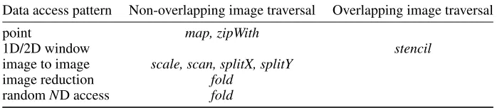
Data access pattern Non-overlapping image traversal Overlapping image traversal
point map, zipWith
1D/2D window stencil
image to image scale, scan, splitX, splitY image reduction fold
[image:4.612.132.481.564.640.2]randomND access fold
1 i m a g e 2 = map i m a g e 1 (\p −> min 255 ( p + 5 0 ) ) ; 2
3 i m a g e 3 = z i p W i t h i m a g e 1 i m a g e 2 (\p1 p2 −> p1 + p2 / 2 ) ; 4
5 i m a g e 4 = z i p W i t h i m a g e 1 [ m a x P i x e l . . ]
6 (\x m a x P i x e l −> i f x > ( m a x P i x e l−50) t h e n p i x e l e l s e 0 ) ; 7
8 b i g g e r I m a g e = s c a l e ( 2 , 3 ) i m a g e 1 ; 9
10 i m a g e 5 = s t e n c i l ( 3 , 1 ) i m a g e 1 (\[ . ] ( x , y ) −> ( [ .−1 ] + [ . ] + [ . + 1 ] ) / 3 ) ; 11
12 i m a g e 6 = s t e n c i l ( 3 , 3 ) i m a g e 1
13 (\p1 p2 p3 p4 p5 p6 p7 p8 p9 ( x , y ) −>
14 a b s ( ( p1 + ( 2∗p2 ) + p3 ) − ( p7 + ( 2∗p8 ) + p9 ) ) 15 + a b s ( ( p3 + ( 2∗p6 ) + p9 ) − ( p1 + ( 2∗p4 ) + p7 ) ) ) ;
Fig. 1: Examples of image processing with stream based skeletons
imreadM,N :ColourT ype→(M:Int)→(N:Int)→I(M,N) mapM,N,A,B:I(M,N)→([P]A→[P]B)→I(M∗(B/A),N)
stencilM,N,A,B:I(M,N)→(A:Int, B:Int)→([P](A∗B)→(Int, Int)→P)→I(M,N) zipW ithM,N,A:I(M,N)→I(M,N)→([P]A→[P]A→[P]A)→I(M,N)
scaleM,N,A,B: (A:Int, B:Int)→I(M,N)→I(M∗A,N∗B) splitXM,N :Int→I(M,N)→(I(M/2,N), I(M/2,N))
splitYM,N :Int→I(M,N)→(I(M,N/2), I(M,N/2)) scanM,N :I(M,N)→Int→(P →Int→Int)→I(M,N)
f oldM,N :State→I(M,N)→(State→Element→[Statement])→State f old:State→Range →(State→Index →[Statement])→State
Fig. 2: RIPL skeletons
RIPL skeletons are reusable generalised image processing patterns, to which the user supplies functions and values. Their distinctions in terms of data access patterns are shown in Table I, with examples given in Fig. 1. Point operations e.g.withmapcomputes a single pixel value from an input pixel, and the processing does not depend on pixel neighbours (line 1 in Fig. 1). Examples include arithmetic, logical and threshold operations. ThezipWithskeleton (line 3) merges two data structures,e.g.two images or combining an image with a stream of a constant value (line 5).
Local operationse.g.withstencildepends on small 1D or 2D sub-regions of neighbouring pixels, e.g.convolution, filtering, smoothing, image enhancements, upsampling an image withscale(line 8) with an interpolation filter withstencil, or horizontally splitting an image withsplitX. For example, splitX 2 img1would return two images, where the first is constructed from columns 1, 2, 5, 6, 9, 10. . . and the second image has columns 3, 4, 7, 8. . . etc.
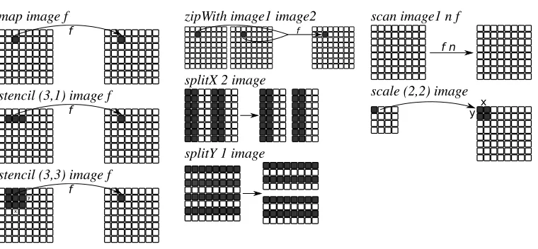
Processing images with RIPL’s stream based skeletons is visualised in Fig. 3. RIPL’s skeleton API is shown in Fig. 2. The user supplies functions and values, using standard notation for function type signatures,e.g. mapis a skeleton that takes two arguments: an M ×N image, and function from a pixel to a pixel, and returns anM ×N image. Images are read withimreadin row major order from left to right, then top to bottom. The typeP represents pixel integer values. An image
map image f f
stencil (3,1) image f f
stencil (3,3) image f f
x y
zipWith image1 image2
f
splitX 2 image
splitY 1 image
scan image1 n f
f n
[image:6.612.110.490.86.262.2]scale (2,2) image x y
Fig. 3: Visualising image processing with RIPL’s stream based skeletons
2.3. Image Stencils, Recursion and Random Access
2.3.1. Image Stencils.RIPL has a primitive for applying 1D and 2D stencils called stencil. It captures a way to express many common image processing kernels such as a blur kernel and edge detection. Thestencilskeleton provides the user with the pixel values, and also the(x, y)position of the centre pixel. Line 10 in Fig. 1 is an implementation of a 1D blur stencil. For 1D stencils, the syntax[.]points to the indexed column wise position of that pixel. Indexing pixels either side is done with+/-,e.g. [.-1]points to the pixel to the left of the[.]pixel. When applying a 2D kernel, e.g. Sobel edge detection on line 12, thestencil (M,N) ..skeleton provides M ∗N pixels to the user defined function. When the user defined kernel is applied at the edges of the image, the closest adjacent pixel is mirrored over the image’s edge. The(x, y)position argument can be used to make a choice about how to compute a kernel result for each position,e.g.applying different kernels for odd and even columns. This functionality is used for separating the low and high bands in a discrete wavelet transform in Section 4.2.3:
img2 = s t e n c i l ( 3 , 1 ) img1 (\[ . ] ( x , y ) −> i f x % 2 == 0
t h e n ( [ . ] − ( ( [ .−1 ] + [ . + 1 ] ) >> 1 ) ) e l s e ( [ . ] + ( ( [ .−1 ] + [ . + 1 ] ) >> 2 ) ) ) ;
2.3.2. Stateful Recursion. Thefoldskeleton is designed to meet algorithmic requirements that do not fit into RIPL’s stream combinator model. This skeleton supports:
— Accumulating state whilst traversingNdimensional data structures including images. — Random access intoNdimensional data structures.
— Recursion with thewhileconstruct.
Thefoldskeleton takes three arguments: 1) an initial state, 2) an iterable data structure, and 3) a user defined function that takes a state and the next element from the structure, then executes a sequence of statements. The initial state can be a boolean or integer literal, a tuple of literals, or N dimensional arrays created withgenarray, where genarray(50,10)creates a50×10array. An iterable data structure can either be a previously computed value, such as an image region, or an iterable range withrange, whererange(10,5)provides the user defined function(i,j)loop counters.
img1 = imread Gray 512 512;
hist = fold genarray(256) img1 (\hist p -> hist[p]++);
sums = scan hist 0 (\elem state -> state+elem);
lut = map sums (\sum -> (sum*255)/(512*512));
img2 = map img1 (\p -> lut[p]);
out img2;
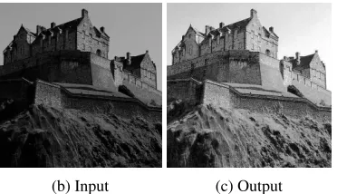
[image:7.612.322.508.92.199.2](a) Dataflow through RIPL code (b) Input (c) Output
Fig. 4: RIPL dataflow analysis of histogram normalisation
m a x P i x e l = f o l d 0 img1 (\maxP p i x e l −> maxP [ 0 ] =max maxP [ 0 ] p i x e l ; ) ; h i s t o g r a m = f o l d g e n a r r a y ( 2 5 6 ) i m a g e 1 (\h i s t p −> h i s t [ p ] + + ; ) ;
The first computes the maximum pixel in an image. The user defined function that applies themax binary operator is folded overimage1, starting from initial state0. The second example instantiates a 1D array of size 256, to serve the purpose of a histogram data structure. The function folds over theimage1, incrementing the bin value positions according to each grayscale pixel value.
2.4. A Dataflow Intermediary for RIPL
RIPL programs are compiled to dataflow process networks (DPNs) [Lee and Parks 2002] as an intermediate representation (IR) of image processing computations. A RIPL program is shown in Fig. 4, which normalises an image’s grayscale distribution with its sum histogram. It reads image pixels withimread, into a histogram withfold. A lookup table containing the scale factor is created withscanandmap. An outputted image is created from this lookup table. The arrows in Fig. 4a show the dataflow analysis that the RIPL compiler performs, to generate pipelined FPGA designs.
RIPL’s dataflow IR comprises static and cyclo-static properties to support the required schedul-ing behaviours of the RIPL skeletons. Synchronous dataflow (SDF) [Lee and Messerschmitt 1987] actors produce and consume the same number of image pixels on every firing. Skeletons map andzipWithare compiled to SDF actors. All other skeletons are compiled to cyclo static dataflow (CSDF) [Bilsen et al. 1996] actors. They have cyclically changing state transition sequences, and have internal actor state for pixel/line buffers to support 1D/2Dstencil,scale,scan,splitX,splitY andfold. The scheduling behaviour of each CSDF actor for RIPL skeletons is fixed, the pixel/line buffer sizes and the functions to produce data output values are derived from the user’s RIPL code. The dataflow IR exploits FPGA parallelism and good data locality:
Parallelism. The dataflow model of independent computational blocks are a natural fit for parallel FPGA circuits, to process infinite image streams. Parallelism is implicit in RIPL, without parallel primitives or pragmas. Generating hardware pipelines hides latency. The RIPL compiler preserves lazy evaluation in the tail of image streams to exploit pipelined parallelism. Otherwise, actors would consume more data than needed to compute their function, which would reduce parallelism and increase memory costs for intermediate storage. There are two forms of automatic RIPL parallelism:
— Temporal parallelism This form of parallelism is introduced when image data is streamed through a pipeline of producer-consumer kernels,e.g.the output from astencilis the input to azipWithoperation.
Data locality.There is no global shared memory in the dataflow model. Instead, the dataflow memory model is that of isolated memory within actors, where computations and their data are co-located. This maps naturally to on-chip contention-free (i.e.parallel accesses) BRAM memory and registers distributed across FPGA fabric.
3. RIPL IMPLEMENTATION
Each RIPL skeleton is compiled to a dataflow actor that encapsulates a Finite State Machine (FSM), responsible for the required scheduling behaviour, and corresponding datapath. These actors are connected into deep parallel pipelines as multiple skeletons are used in larger programs. RIPL enforces single assignment semantics, i.e.a variable is assigned a value with a skeleton instance exactly once. This makes data dependencies easy to extract to dataflow wiring, to facilitate the gen-eration of hardware pipelines. The RIPL compiler is open source1, and the RIPL, CAL and C++ implementations for the evaluation in Section 4 are available as an open dataset [Stewart 2018].
3.1. Skeletons to Dataflow FSMs
3.1.1. Dataflow Semantics for RIPL Skeletons.The compilation of each RIPL skeleton is based on a framework for describing rule based dataflow actors [Janneck 2003]. It describes the data rates and static scheduling for each RIPL skeleton in terms of transitions on an abstract machine, which is later compiled to hardware specified in Verilog (Section 3.2). An actor is a sequential process, communicating values by transitioning between states in the actor’s FSM. The state machine re-ceives tokens and reacts to them, possibly entering another state, and possibly producing tokens. A state transition fromσtoσ0 consumes a tuplesof token sequences and produces a tuples0 of to-ken sequences. An actor has a set ofminput ports, writtenSm, andnoutput ports, writtenSn. The valuemis dictated by the arity of the corresponding RIPL skeleton,e.g. zipWithtakes two images as inputs and hencemis 2 for this skeleton. If the output of one skeleton is used as an input argument of multiple other skeletons, then those actors are connected to the same input port and the stream is automatically duplicated into each connection.
LetU be the universe of all values, andS =U∗be the set of all finite sequences inU. A tuple
s∈Smcontains one or more token sequences consumed frompports, where1
6p6m. We write
spAto describe a token sequence of lengthAat portp. For example, a transition fromσtoσ0 that consumes sequences from input ports 1 and 2 of lengthsAandB, to produce a sequence of length
Cto an output port 1 is written as:
σ s
1 A×s2B7→s
01 C
−−−−−−−−→σ0
For some scheduling phases of a RIPL skeleton, a transition rule may not read from or write to any ports. We use∅as port descriptions for these transitions. To support the stateful RIPL skeletons such asstencil, internal actor state is needed. We addSas a notation to transition rules for internal actor state. State transition examples are written as follows:
hσ0,Si
s137→s01 6
−−−−−→ hσ1,S0i
This transition moves from FSM stateσ0 with a set of internal variable states inS, to FSM state
σ1with internal variable statesS0, and consumes three input tokens from input port 1 and emits six
output tokens to output port 1. In the mapping from RIPL to dataflow graphs, the vertices (actors) represent image operations and the edges (wires) represent dataflow between composed skeletons.
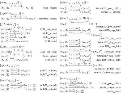
3.1.2. Compilation scheme.
Pointwise skeletons.The skeleton to dataflow FSMs compilation scheme is in Fig. 5. Each skele-ton is compiled to an actor with one or more transitions. ThemapandzipWithskeletons are each
JmapM,N,A,BfK=
hσ0,{}i
f:s1A7→s01B
−−−−−−−−→ hσ0,{}i (map stream)
JzipW ithM,N,AfK=
hσ0,{}i
f:s1A×s2A7→s01A
−−−−−−−−−−−→ hσ0,{}i (zipWith stream)
Jf old state fK=
hσ0, statei f:s1
17→∅
−−−−−−→ hσ1,Si (fold init state)
hσ1,Si f:s1
17→∅
−−−−−−→σ1,S0
(fold accum)
hσ1,Si ∅7→s011
−−−−→ hσ2,Si (fold output)
hσ2,Si ∅7→∅
−−−→ hσ0, statei (fold reset)
JscanM,N state fK=
hσ0, statei f:s1
17→∅
−−−−−−→ hσ1,Si (scan init state)
hσ1,Si
f:s117→s011
−−−−−−−→σ1,S0 (scan output)
hσ1,Si ∅7→∅
−−−→ hσ0, statei (scan reset)
JsplitXM,N,AK=
hσ0,{}i s1
A7→s 01
A
−−−−−−→ hσ1,{}i (splitX output1)
hσ1,{}i s1A7→s02A
−−−−−−→ hσ0,{}i (splitX output2)
JsplitYM,N,AK=
hσ0,{}i s1
A∗M7→s 01
A∗M
−−−−−−−−−−→ hσ1,{}i (splitX output1)
hσ1,{}i
s1A∗M7→s02A∗M
−−−−−−−−−−→ hσ0,{}i (splitX output2)
JstencilM,N,A(A,1)fK=
hσ0,{}i
s1(A−1)7→∅
−−−−−−−→ hσ1,Si (stencil1D pop buffer)
hσ1,Si f:s1
17→s 01
1
−−−−−−−→σ1,S0
(stencil1D stream)
JstencilM,N,A,B(A, B)kK=
hσ0,{}i
s1((B−1)∗M+A)7→∅
−−−−−−−−−−−−−→ hσ1,Si
(stencil2D pop buffer) hσ1,Si
k:s117→s011
−−−−−−−→σ2,S0 (stencil2D top left)
hσ2,Si
k:s1(M−2)7→s01(M−2)
−−−−−−−−−−−−−−−→σ3,S0
(stencil2D top row) hσ3,Si
k:s117→s011
−−−−−−−→σ4,S0
(stencil2D top right)
hσ4,Si
k:s117→s011
−−−−−−−→σ5,S0
(stencil2D mid left)
hσ5,Si
k:s1(M−2)7→s01(M−2)
−−−−−−−−−−−−−−−→σ6,S0 (stencil2D mid)
hσ6,Si
k:s117→s011
−−−−−−−→σ7,S0 (stencil2D mid right)
hσ7,Si
k:s117→s011
−−−−−−−→σ8,S0
(stencil2D bottom left)
hσ8,Si k:s1
(N−2)7→s 01
(M−2)
−−−−−−−−−−−−−−−→σ9,S0
(stencil2D bottom row) hσ9,Si
k:s117→s011
−−−−−−−→ hσ0,{}i (stencil2D bottom right)
JscaleM,N,A,BK=
hσ0,{}i s1
A7→s 01
M∗A
−−−−−−−−→ hσ1,Si (scale pop buffer)
hσ1,Si
∅7→s01M∗(B−1)
−−−−−−−−−−→ hσ1,Si (scale output row)
hσ1,Si ∅7→∅
[image:9.612.115.513.96.397.2]−−−→ hσ0,{}i (scale reset)
Fig. 5: Compilation scheme from RIPL skeletons to actor FSMs
compiled to a single transition rule in an SDF actor with no internal state, i.e. transition rules (map stream) and(zipWith stream) map from an empty internal state {} to an empty internal state, and the output values from these transitions are determined by the user defined functionf.
Image Transforms.The scale skeleton is compiled to three transition rules. The (scale pop buffer) consumes a row and outputs each pixel in turn by the width scale factor
M. The(scale output row)outputs this scaled rowN −1 times, where N is the height scale factor, then the FSM is reset toσ0with transition(scale reset). Thescanskeleton is compiled to
three transition rules. The(scan init state)rule initialises the actor buffer with the user defined initial state. The(scan output)rule performs the accumulation operation, outputting intermediate values until a data structure is consumed, then (scan reset) reset back to the initial state. The splitXskeleton has two rules, one each for outputting to output ports 1 and 2. TakesplitX 2 image, (splitX output1)consumes 2 tokens then outputs them to output port 1, then(splitX output2)does the same, outputting to output port 2. This alternating schedule repeats forever. The same FSM schedule is used forsplitY, this time consuming entire rows in each transition.
Stencils. A 1D image blur stencil in Fig. 6 demonstrates how the RIPL compiler minimises the memory requirements of an FPGA. The compiler infers the range of the indexed pixel either side of [.], which in this case is 3 pixels between[.−1]and[.+ 1]. The actor contains a 3 element array that acts as a circular buffer, which is partially filled with 2 elements by firing rule (sten-cil1D pop buffer) to reach stateσ1 and a mid position pointer is set to1. Each time the
index
0
1 2
[.]
+1 -1
midpoint
new pixel
output pixel
stencil (3,1) image (\[.] (x,y) -> ([.-1] + [.] + [.+1]) / 3)
Fig. 6: Circular buffer to supportstencil (3,1) ..for a 1D blur kernel
RIPL function is computed on the buffer’s contents as the output token value, and the mid position pointer is rotated forward one position. This stencil actor needs memory for just four pixels, three element circular buffer and the incoming token, to apply a 1D blur over an entire image.
Thestencilskeleton for 1D stencils is compiled to two transition rules. Internal state for 1D sten-cils is populated with the(stencil1D pop buffer)rule before transitioning to stream based rules (stencil1D stream). The stencilskeleton for 2D stencils is compiled to 10 transition rules. The (stencil2D populate buffer)rule consumes the first two rows andApixels required to start pro-cessing an image from the top left corner,i.e.by consuming((B−1)∗M +A)tokens whereA
andBare the width and height of the kernel window andM is the width of the entire image. The remaining 9 rules carry out three tasks:1)consume one pixel into internal state, 2)compute the application of the user defined 2D kernel functionf on the window around the central pixel, and3) output that computed value. They are defined as separate transition rules to index the internal state to handle boundary conditions at image edges, where the edge pixel is mirrored over the boundary.
Reductions and Stateful Recursion. Thefoldskeleton is compiled to four transition rules. Internal actor state is persisted throughout the consumption of each input data structure,e.g.an image region. The internal state buffer is initialised with the user definedstatevalue, before being modified each firing with(fold accum). Once an entire data structure is consumed, the(fold output)rule begins firing to output the final state. The(fold reset)resets the internal actor buffer to the initial state and readies the actor to consume the next data structure.
zipWithimage1 image2 (λp1 p2→(p1 + p2) / 2)
hσ0,{}i
[3]×[43]7→[23]
−−−−−−−−→ hσ0,{}i (zipWith stream)
hσ0,{}i
[4]×[8]7→[6]
−−−−−−−→ hσ0,{}i (zipWith stream)
hσ0,{}i
[16]×[8]7→[12]
−−−−−−−−→ hσ0,{}i (zipWith stream)
hσ0,{}i
[62]×[48]7→[55]
−−−−−−−−−→ hσ0,{}i (zipWith stream)
hσ0,{}i
[30]×[10]7→[20]
−−−−−−−−−→ hσ0,{}i (zipWith stream)
hσ0,{}i
[12]×[92]7→[52]
−−−−−−−−−→ hσ0,{}i (zipWith stream)
fold0 image1 (λmaxPixel pixel→
maxPixel[0] = max maxPixel[0] nextPixel)
hσ0,0i [8]7→∅
−−−−→ hσ1,8i (fold init state)
hσ1,8i [5]7→∅
−−−−→ hσ1,8i (fold accum)
hσ1,8i [9]7→∅
−−−−→ hσ1,9i (fold accum)
hσ1,9i [16]7→∅
−−−−→ hσ1,16i (fold accum)
hσ1,16i
∅7→[16]
−−−−→ hσ2,0i (fold output)
hσ2,0i
∅7→∅
−−−→ hσ0,0i (fold reset)
Fig. 7: RIPL skeleton transition execution examples
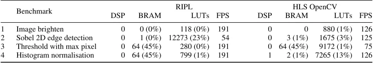
Benchmark RIPL HLS OpenCV
DSP BRAM LUTs FPS DSP BRAM LUTs FPS
1 Image brighten 0 0 (0%) 118 (0%) 191 0 0 880 (1%) 126
[image:11.612.117.499.94.159.2]2 Sobel 2D edge detection 0 1 (0%) 12273 (23%) 54 0 3 (1%) 1675 (3%) 125 3 Threshold with max pixel 0 64 (45%) 280 (0%) 191 0 64 (45%) 9172 (1%) 75 4 Histogram normalisation 0 64 (45%) 799 (1%) 191 1 2 (1%) 7265 (13%) 126
Table II: Micro Benchmark Results
pixels have been consumed, the internal state is outputted with (fold output), before the FSM is reset tohσ0,0ifor the next image frame.
3.2. Dataflow to FPGAs
The CAL dataflow language [Eker and Janneck 2003] is the target language of RIPL’s dataflow IR backend. There are three phases to compile RIPL to FPGAs: 1) compiling RIPL to CAL, 2) compiling the dataflow graph to Verilog, and 3) synthesising the Verilog to a bitfile. The dataflow intermediary provides optimisation opportunities,e.g. [Stewart et al. 2017], before being compiled to hardware components like registers, memories and actor communication handshake protocols. Xronos [Bezati 2015], an FPGA backend plugin for the Orcc compiler, maps each actor into a language independent model (LIM) and connects each LIM block to a clock. Xronos is designed to support dynamic asynchronous dataflow, and therefore adds a FIFO based data communication mechanism to support token passing. Decoupling actor communication via these FIFOs results in 2 clock cycles latency per pixel,i.e.for a 512x512 image at 100MHz the highest theoretical perfor-mance is 512100000000×512×2 = 191FPS for a single actor performing elementwise operations. The Xilinx OpenForge compiler allocates hardware: memory, arithmetic datapaths, registers and actor intercon-nects, then generates HDL modules for each actor and for defining dataflow connectivity between these modules. This HDL code is synthesised and deployed to FPGAs using commercial tools.
RIPL’s code generation strategy maximises spatial parallelism to maximise the number of opera-tions per clock cycle. By default, OpenForge uses BRAM blocks for CAL arrays beyond a certain size. Our experiments with OpenForge show that a BRAM block is instantiated for CAL arrays requiring more than 2KB of storage,e.g.about a4×512row buffer at 8 bits per pixel. To use a BRAM in the combinational setting, at most two read/write accesses to a CAL array may occur. When more than 2 reads/writes are performed on the same array in an actor’s action, OpenForge instead instantiates LUTs for CAL arrays with 3+ reads/writes to preserve zero latency accesses.
4. EVALUATION
4.1. RIPL versus HLS OpenCV
4.1.1. Expressivitiy. Vivado HLS OpenCV [Stephen Neuendorffer and Wang 2015] is a collec-tion of 34 predefined funccollec-tions, a subset of the 2,500+ algorithm funccollec-tions in OpenCV for CPUs. An example is in Fig. 8. In contrast, RIPL provides algorithmic templates, whose functionality is entirely user defined. For example, the HLS OpenCVhls::Maxfunction for combining two images can be expressed with RIPL’szipWith. HLS OpenCV’shls::Filter2Dis a convolution filter. RIPL’s stencilsupports any stencil function, including convolution. This demonstrates the inflexibility of libraries of fixed kernels. Moreover, the library approach prohibits optimisations across library call boundaries. Other expressivity differences are:
1 hls::Mat<512,512, HLS_8UC1> img_0(rows,cols); 2 hls::Mat<512,512, HLS_8UC1> img_1(rows,cols); 3 hls::Mat<512,512, HLS_8UC1> img_2(rows,cols); 4 hls::Mat<512,512, HLS_8UC1> img_3(rows,cols); 5
6 // explicit depth for img_2 to prevent deadlock
7 #pragma HLS stream depth=262144 variable=img_2.data_stream 8
9 // convert AXI4 stream data to hls::mat format 10 hls::AXIvideo2Mat(INPUT_STREAM1, img_0); 11
12 // duplicate the img_0 stream 13 hls::Duplicate(img_0,img_1,img_2); 14
15 // find the maximum pixel of img_1 duplicate 16 int maxP, minP;
17 hls::Point p1,p2;
18 hls::MinMaxLoc(img_1,&minP,&maxP,p1,p2); 19
20 // threshold the img_2 duplicate using the max pixel - 50 21 int threshold = maxP - 50;
22 hls::Threshold(img_2,img_3,threshold,255,HLS_THRESH_TOZERO);
Fig. 8: Thresholding with a maximum pixel value in HLS OpenCV
— Image shape inference OpenCV programming requires explicit dimension in image declara-tions,e.g.hls :: M ath512,512, HLS 8U C1idefines a512×512single channel image, using 8 unsigned bits per pixel. In contrast, the RIPL compiler infers the dimension of every intermedi-ate image, by following dimension transformations performed by skeletons through the implicit dataflow paths starting fromimread, where dimensions are specified.
— Parallel pipelines Pipelining in RIPL is automatic, e.g. streaming the result of a map in a stencil will generate a hardware pipeline. In HLS OpenCV, the programmer must specify #pragma HLS dataflowabove the function calls intended to be pipelined over the image stream.
4.1.2. Performance Comparison.We use four benchmarks to compare the space performance of RIPL and OpenCV compiled to FPGAs using Vivado HLS [Xilinx 2017b]. Programs are compiled for the Xilinx Zedboard XC7Z020 for 512×512 single channel images. The post place-and-route results in Table II are taken from [Stewart et al. 2016]. To quantify computational image processing performance, we use RTL simulation to calculate latency in clock cycles per512×512frame and report frames per second (FPS) according to the clock frequency. All experiments were performed using a 100MHz clock, which is the default frequency for Vivado HLS, and we did not perform any speed optimisations on Vivado HLS or RIPL-generated code.
HLS OpenCV uses less BRAM than RIPL for histogram normalisation. The dataflow graph gen-erated from RIPL computes two passes of the image, one to compute the histogram and a second to normalise the colour distribution with it. In contrast,hls::EqualizeHist()normalises a frame using a histogram computed for the previous frame. This approximation optimisation means that BRAM is not needed to store an image for the second pass to normalise with the computed histogram.
4.2. Higher Level Case Study 1: Visual Saliency
This section uses a pyramidal visual saliency algorithm to compare the performance of RIPL ver-sus variants of a C++ equivalent implementation compiled with Vivado HLS. The algorithm com-prises three components: 1) an average filter (Section 4.2.1), 2) a discrete wavelete transform (Sec-tion 4.2.2), and 3) a weighted linear summa(Sec-tion of wavelet subbands (Sec(Sec-tion 4.2.3).
4.2.1. Low Level Image Processing: Average Filtering. Average filtering is one of the most com-monly used filtering methods used in image pre-processing that helps to reduce the amount of in-tensity variation between a pixel and its neighbours. Each pixel value is replaced with a mean of its neighbours including the pixel itself and commonly realised by convolving with a predefined mask [Gonz´alez and Woods 1992]. An equation for such filters is expressed as below:
I0 =W ∗I=
N X
n=1
M X
m=1
w(m, n)·I(m, n), (1)
whereIis the input image of sizeM ×N,I0is filtered image,W is the filter kernel,mandnare
the pixel locations and∗is a convolution operator. The process is repeated using a sliding window to receive filter output for entire image. Average filtering with filter coefficientsw(m, n) = 1
9 can
be implemented as a RIPL function using thestencilskeleton:
l e t a v e r a g e F i l t e r i m a g e =
b l u r r e d I m a g e = s t e n c i l ( 3 , 3 ) i m a g e
(\p1 p2 p3 p4 p5 p6 p7 p8 p9 ( x , y ) −> ( p1+p2+p3+p4+p5+p6+p7+p8+p9 ) / 9 ) ; b l u r r e d I m a g e ;
4.2.2. Intermediate Level Image Processing: Multi Resolution 2D Wavelet Transform. The dis-crete wavelet transform (DWT) is used for many image processing applications,e.g.compression, de-noising and texture analysis. Multi-orientation and multi resolution analysis using DWT closely resembles human vision. DWT decomposes an image into independent frequency subbands of mul-tiple orientations at mulmul-tiple scales demonstrating details and structures. Due to its popularity in the JPEG2000 image compression standard [Taubman and Marcellin 2012], we use the 5/3 wavelet ker-nel as our RIPL example, using a lower complexity lifting-based approach. The filters are realised by decomposing the signal into lifting steps by factoring its polyphase matrix using the Euclidean factoring algorithm [Daubechies and Sweldens 1998]. The input signal, lowpass subband signal, and highpass subband signal are denoteda[n],s[n]andd[n]respectively. DWT is expressed in Eq. (2), wheres0[n],a[2n]andd0[n],a[2n+ 1]:
5/3
d[n] =d0[n]−21(s0[n+ 1] +s0[n]),
s[n] =s0[n] +41(d[n] +d[n−1]).
(2)
A 2D DWT is computed by separately filtering rows and columns leading to one approximation (LL) subband & three detailed subbands in the decomposition level i ∈ N1 emphasising
verti-cal (LHi), horizontal (HLi) and diagonal (HHi) contrasts within an image, portraying prominent
edges in various orientations as shown in Fig. 9. This process is repeated on the LL subband to get multiresolution decomposition. The 5/3 DWT is implemented as a RIPL function in Fig. 10. TheL
andH components of the inputimageare computed withstencilon line 2 and them separated to
(a) DWT illustration (b) LL1 (c) LH1 (d) HL1 (e) HH1
Fig. 9: An example of multiresolution wavelet decomposition, where (b), (c), (d) and (e) are level 1 approximation (LL1), vertical (LH1), horizontal (HL1) and diagonal (HH1) subbands.
1 l e t w a v e l e t D e c o m p o s e i m a g e =
2 img2 = s t e n c i l ( 3 , 1 ) i m a g e (\[ . ] ( x , y ) −>
3 i f x % 2 == 0 t h e n ( [ . ] − ( ( [ .−1 ] + [ . + 1 ] ) >> 1 ) ) 4 e l s e ( [ . ] + ( ( [ .−1 ] + [ . + 1 ] ) >> 2 ) ) ) ; 5 ( L , H) = s p l i t X 1 img2 ;
6 img3 = s t e n c i l ( 3 , 3 ) L (\p1 p2 p3 p4 p5 p6 p7 p8 p9 ( x , y ) −> 7 i f y % 2 == 0 t h e n ( p2 + p6 ) >> 2 e l s e ( p2 − p6 ) >> 1 ) ; 8 img4 = s t e n c i l ( 3 , 3 ) H (\p1 p2 p3 p4 p5 p6 p7 p8 p9 ( x , y ) −> 9 i f y % 2 == 0 t h e n ( p2 + p6 ) >> 2 e l s e ( p2 − p6 ) >> 1 ) ; 10 ( LL , LH ) = s p l i t Y 1 img3 ;
11 ( HL , HH) = s p l i t Y 1 img4 ; 12 ( LL , LH , HL , HH) ;
Fig. 10: 5/3 Discrete Wavelet Transform in RIPL
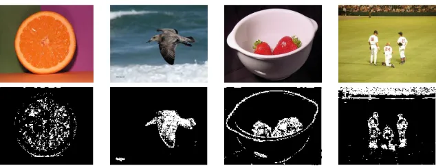
Fig. 11: Example saliency maps computed by the original model: row 1 is the original image, and row 2 shows the thresholded saliency map generated by our implementation.
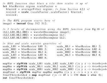
4.2.3. High Level Image Processing: Visual Saliency Modelling.The human visual system is sen-sitive to many salient features that lead to attention being drawn towards specific regions in a scene. A visual attention model identifies the salient regions in an image as perceived by human vision and has applications in many domains including computer vision [Borji and Itti 2013]. We have adopted the visual attention model from in [Bhowmik et al. 2016], which demonstrates superior performances in joint saliency detection and low computational complexity. The algorithm uses the 5/3 DWT in Section 4.2.2 as its core decomposition. Example algorithm results are shown in Fig. 11. DWT captures horizontal, vertical and diagonal contrasts within an image, respectively, portray-ing prominent edges in various orientations. A complete visual saliency RIPL implementation is shown in Fig. 12, which uses thewaveletDecomposeRIPL function from Fig. 10. It processes the
[image:14.612.149.466.365.486.2]1 /∗ RIPL f u n c t i o n t h a t b l u r s a t i l e t h e n s c a l e s i t up ∗/
2 l e t b l u r R e s i z e r e g i o n s c a l e F a c t o r =
3 b l u r r e d = a v e r a g e F i l t e r r e g i o n ; /∗ f r o m S e c t i o n 4.2.1 ∗/
4 r e s i z e d = s c a l e ( s c a l e F a c t o r , s c a l e F a c t o r ) b l u r r e d ; 5 r e s i z e d ;
6
7 /∗ The RIPL p r o g r a m s t a r t s h e r e ∗/
8 i m a g e 1 = imread Gray 512 5 1 2 ; 9
10 /∗ 3 l e v e l s o f d e c o m p o s i t i o n u s i n g t h e RIPL f u n c t i o n f r o m Fig. 10 ∗/
11 ( LL1 , LH1 , HL1 , HH1 ) = w a v e l e t D e c o m p o s e i m a g e 1 ; 12 ( LL2 , LH2 , HL2 , HH2 ) = w a v e l e t D e c o m p o s e LL1 ; 13 ( LL3 , LH3 , HL3 , HH3 ) = w a v e l e t D e c o m p o s e LL2 ; 14
15 /∗ b l u r and s c a l e w a v e l e t q u a r t i l e s ∗/
16 scale LH1 = b l u r R e s i z e LH1 2 ; scale HL1 = b l u r R e s i z e HL1 2 ; 17 scale HH1 = b l u r R e s i z e HH1 2 ; scale LH2 = b l u r R e s i z e LH2 4 ; 18 scale HL2 = b l u r R e s i z e HL2 4 ; scale HH2 = b l u r R e s i z e HH2 4 ; 19 scale LH3 = b l u r R e s i z e LH3 8 ; scale HL3 = b l u r R e s i z e HL3 8 ; 20 scale HH3 = b l u r R e s i z e HH3 8 ;
21
22 mapVer = z i p W i t h scale LH1 scale LH2 scale LH3 (\x y z −> 4∗x +8∗y +4∗z ) ; 23 mapHor = z i p W i t h scale HL1 scale HL2 scale HL3 (\x y z −> 4∗x +8∗y +4∗z ) ; 24 mapDia = z i p W i t h scale HH1 scale HH2 scale HH3 (\x y z −> 4∗x +8∗y +4∗z ) ; 25 m a p F i n a l = z i p W i t h mapVer mapHor mapDia (\x y z −> x + y + z ) ;
[image:15.612.101.474.92.381.2]26 f i n a l T h r e s h o l d e d = map m a p F i n a l (\x −> i f x > 150 t h e n x e l s e 0 ) ; 27 o u t f i n a l T h r e s h o l d e d ;
Fig. 12: Visual saliency in RIPL
weight in the original algorithm. The RIPL implementation applies three levels of wavelet decom-position. Due to the dyadic nature of the multi-resolution wavelet transform, the image resolutions are decreased after each wavelet decomposition iteration from lines 11 to 13. This is useful in cap-turing both short and long structural information at different scales. TheblurResizefunction on line 2 is called on lines 16 to 20, which applies an average filter to each subband to remove unnecessary finer details, then scales up the result back to a full resolution output. The interpolated subband fea-ture maps,lhi(horizontal),hli(vertical) andhhi(diagonal),i∈N1, for all decomposition levelsL
1 to 3 are combined by a weighted linear summation as illustrated in Eq. (3):
lh1···LY = L X
i=1
lhi∗τi hl1···LY = L X
i=1
hli∗τi, hh1···LY = L X
i=1
hhi∗τi (3)
whereτi is the subband weighting parameter andlh1···LY,hl1···LY andhh1···LY are the subband
feature maps for the spectral channelY, on lines 22 to 24.
LastlySY, the saliency map for theY spectral channel, is on line 25 and is computed as below,
before being thresholded with a binary threshold to emphasise salient regions:
SY =lhY +hlY +hhY. (4)
4.2.4. Visual Saliency Results.
in-FPS unroll BRAM DSP FF LUT Benchmark factor (/2060) (/2800) (/607200) (/303600)
RIPL 71 - 1% 0% 2% 18%
C++ 21 - 90% 1% 1% 1%
C++with array reuse 23 4 12% 1% 1% 1%
C++with array reuse 24 8 12% 2% 1% 6%
C++with array reuse 28 16 12% 4% 3% 12%
C++with array reuse 28 32 12% 9% 6% 23%
C++with array reuse 27 64 12% 18% 45% 60%
[image:16.612.140.474.93.215.2]C++with array reuse 25 96 12% 25% 94% (103%)
Table III: Visual saliency on a Virtex 7
place in the body of each function. These template parameters are propagated through the program at compile time from512and512height and width image dimensions in the test bench,e.g.
t e m p l a t e<i n t h , i n t w> v o i d b l u r F i l t e r ( u c h a r i m a g e [ h ] [ w ] ) ;
The C++ variants are:
(1) C++ with array reuse. Each function contains declared 2D arrays with element values initialised to zero, e.g. lowBand[h][w/2] and highBand[h][w/2] are declared in the waveletDecompose function, which can both be populated in a single loop statement to separate the low and high bands in one iteration over the image. This version contains 27 arrays.
(2) C++ with extensive reuse of arrays. This version reuses some arrays for different purposes. Refactoring has been done manually,e.g.renaminglowBand[h][w/2]toband[h][w/2]and pop-ulating it with low band FWT values to compute LL and LH, before re-poppop-ulating it with high band values to compute HL and HH. This approach also sequentialises the summation of weighted LH, HL and HH contrasts because one array is repopulated with LH, then HL, then HH, after each sum accumulation into an output array. This version contains 13 arrays.
(3) C++ with array reuse and loop unrolling. Loop unrolling with#pragma AP unrollis employed to create multiple parallel independent operations from originally sequential loops. This loop unrolling pragma is used in 8 places, and the unrolling factor is varied to measure the trade off between space and latency.
Hardware designs for RIPL and C++ are clocked at 100MHz for the Virtex 7 VC707 and syn-thesised using Vivado 2016.2. Results are displayed in Table III. Vivado HLS does not apply fusion optimisations to eliminate intermediateforloops over successive arrays, hence the 90% BRAM use for 27 image buffers. Manually eliminating intermediate arrays down to 13 reduces BRAM use to 12%, which runs at 23 FPS. Unrolling the 8forloops in the C++ code upto an unroll factor of 32 increases FPS to 28, as well as increasing DSP, FF and LUT resource use. FPS performance de-grades as more space is needed with a 64 unroll factor, and an unroll factor of 96 requires too many LUTs. The RIPL program achieves 2.5x higher FPS performance than the best C++ variant at 71 FPS, using fewer BRAMs and a similar number of LUTs.
RIPL versus dataflow in software.The RIPL program has also been compiled for an Intel i5 3.2GHz CPU, using the Orcc dataflow compiler’s C backend. This CPU is a high end processor com-pared to embedded processors usually used for remote image processing. The CPU visual saliency performance is 9 FPS. The FPGA performance is 8.3x faster than the CPU.
in a program that is 111x shorter than its direct dataflow program equivalent. The Orcc compiler generates approximately 26k lines of C and 356k lines of Verilog. These program sizes are much larger because it combines both algorithm code and scheduling code to implement DPN actor firing semantics and actor synchronisation on dataflow wires.
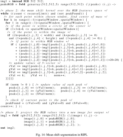
4.3. Higher Level Case Study 2: Mean Shift Segmentation
The mean shift clustering algorithm [Fukunaga and Hostetler 1975] is a method to cluster data. This has been applied to text detection in images [Kim et al. 2003] and real time video tracking of non-rigid objects [Comaniciu et al. 2000]. Because the algorithm is used to distinguish between objects based on their colour rather than shape, non-rigid objects can be tracked. The applications in image segmentation were proposed in [Comaniciu and Meer 1999].
4.3.1. Mean Shift Segmentation Algorithm.Each pixel is mapped into an RGB colour space, where each pixel has a vector position according to its red, green and blue values. This feature space can be regarded as the probability density function of colour. Dense regions of this space correspond to the local maxima of the probability density function. The value of a density function at a point are estimated from the values observed around that point. The multivariate kernel density estimator at the pointxestimates the value using points within radiushofxand is given by;
ˆ
fh,k(x) = ck nhd
n X
i=1
k(x−xh i
2
). (5)
The density gradient estimator at a point can be estimated similarly from the values within a small window around the point. The modes of the density estimator are found at the points with zero gradient`
f(x) = 0. The mean-shift vector given by
mh,k(x) =
1 2h
2cˆ
` fh,k(x)
ˆ fh,−k0(x)
= Pn
i=1xik0(||x−xh i||2) Pn
i=1k0(||
x−xi
h ||2)
−x, (6)
is the difference between the weighted mean of points within the bandwidth parameterhandx, the center of the window. It points in the direction of a normalised maximum density gradient estimate; it is zero at the point where the gradient of the probability density function is zero. The mean shift vector can therefore be used to define a path towards the local maximum of the estimated density for each point in the feature space. To ensure that mean shift clustering is applied only to neighbouring image pixels of similar RGB colours, the mean shift vector is rewritten:
mhr,hs,G(x) = Pn
i=1x
r,s i k0(||
xr−xr i hr ||
2)k0(||xs−xs i hs ||
2)
Pn i=1k0(||
xr−xr i hr ||
2)k0(||xs−xsi hs ||
2) −x, (7)
wherexr,sis the 5D position in the joint-space,xris the 3D component of the joint space vector corresponding to the range andxsis the 2D component of the joint-space vector corresponding to
the position in the image. Using the Epanechnikov kernel, the required value;
−k0(x−x
0
h ) =
1 0≤x−x0≤h
0 x−x0> h, (8)
determines that all pointsx0within a radiushofxare considered in the calculation, and all points outside are not. The algorithm is in Algorithm 1. For each point in the joint space;
(1) Define a spherical window of radius hr around the 3 colour dimensions of this point and a
circular window of radiushsaround the spatial dimensions and calculate the mean shift vector
(equation 7) from this point;
All points with the same peak are considered to belong to the same cluster.
Algorithm 1Mean-Shift clustering algorithm pseudocode input :Image file
output:Image with each cluster shaded the colour of its peak
1 foreach index in joint space arraydo
2 whilepeak has not been found & iteration limit not exceededdo 3 Collect points within the spatial window
4 Collect points within the range window 5 Calculate mean-shift vector using equation 7 6 ifmean shift vector is zerothen
7 Peak has been found
8 end
9 Add mean shift vector to current point in joint space 10 end
11 Store value of peak in equivalent index of output image 12 end
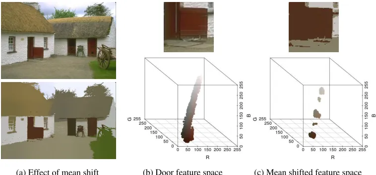
Mean shift segmentation of image #385028 from the Berkeley Segmentation training Dataset [Martin et al. 2001] is shown in Fig. 13. Fig. 13b shows the feature space for the red door, Fig. 13c shows the segmented colours in the feature space after mean shift.
[image:18.612.114.493.343.519.2](a) Effect of mean shift (b) Door feature space (c) Mean shifted feature space
Fig. 13: Mean Shift Segmentation Visualised
/∗ p h a s e 1 : map RGB i m a g e i n t o a 5D a r r a y f o r RGB + f e a t u r e s p a c e d a t a ∗/
img1 = imread RGB 512 5 1 2 ;
peaksRGB = f o l d g e n a r r a y ( 5 1 2 , 5 1 2 , 5 ) r a n g e ( 5 1 2 , 5 1 2 ) (\( p e a k s ) ( i , j ) −>
/∗ p h a s e 2 : t h e mean s h i f t k e r n e l o v e r t h e RGB f e a t u r e s s p a c e ∗/
w h i l e ( ( c o u n t < r e c u r s e L i m i t ) and ( n o t p e a k F o u n d ) ) {
/∗ f o r e a c h p o i n t w i t h i n c h o s e n window , f i n d c e n t e r o f mass ∗/
f o r k i n r a n g e ( (−1 )∗s p a t i a l W i n d o w , s p a t i a l W i n d o w ) {
f o r l i n r a n g e ( (−1 )∗s p a t i a l W i n d o w , s p a t i a l W i n d o w ) {
/∗ i f t h e p o i n t i s w i t h i n a c i r c l e o f t h e c e n t e r ∗/
i f ( l∗l +k∗k <= s p a t i a l W i n d o w∗s p a t i a l W i n d o w ){
/∗ i f t h e p o i n t i s w i t h i n t h e i m a g e ∗/
i f ( ( k+ p e a k s [ i , j , 3 ] < w i d t h ) and ( k+ p e a k s [ i , j , 3 ] >= 0 ) and ( l + p e a k s [ i , j , 4 ] < h e i g h t ) and ( l + p e a k s [ i , j , 4 ] >= 0 ) ) {
/∗ i f p o i n t i s w i t h i n RGB window ∗/
i f ( ( p e a k s [ i , j ,0]−img1 [ p e a k s [ i , j , 3 ] + k , p e a k s [ i , j , 4 ] + l , 0 ] )
∗ ( p e a k s [ i , j ,0]−img1 [ p e a k s [ i , j , 3 ] + k , p e a k s [ i , j , 4 ] + l , 0 ] ) + ( p e a k s [ i , j ,1]−img1 [ p e a k s [ i , j , 3 ] + k , p e a k s [ i , j , 4 ] + l , 1 ] )
∗ ( p e a k s [ i , j ,1]−img1 [ p e a k s [ i , j , 3 ] + k , p e a k s [ i , j , 4 ] + l , 1 ] ) + ( p e a k s [ i , j ,2]−img1 [ p e a k s [ i , j , 3 ] + k , p e a k s [ i , j , 4 ] + l , 2 ] )
∗ ( p e a k s [ i , j ,2]−img1 [ p e a k s [ i , j , 3 ] + k , p e a k s [ i , j , 4 ] + l , 2 ] )<=20∗20) {
/∗ u p d a t e v a l u e s o f 5−v e c t o r ∗/
r V a l += img1 [ p e a k s [ i , j , 3 ] + k , p e a k s [ i , j , 4 ] + l ,0]−p e a k s [ i , j , 0 ] ; g V a l += img1 [ p e a k s [ i , j , 3 ] + k , p e a k s [ i , j , 4 ] + l ,1]−p e a k s [ i , j , 1 ] ; b V a l += img1 [ p e a k s [ i , j , 3 ] + k , p e a k s [ i , j , 4 ] + l ,2]−p e a k s [ i , j , 2 ] ; x V a l += k ; y V a l += l ; norm + + ;
}}}}}
i f ( norm ! = 0 ) { /∗ u p d a t e v a l u e o f e a c h p e a k ∗/
p e a k s [ i , j , 0 ] += ( r V a l / norm ) ; p e a k s [ i , j , 3 ] += ( x V a l / norm ) ; p e a k s [ i , j , 1 ] += ( g V a l / norm ) ; p e a k s [ i , j , 4 ] += ( y V a l / norm ) ; p e a k s [ i , j , 2 ] += ( b V a l / norm ) ;
}
/∗ c h e c k i f c u r r e n t p o i n t i s t h e p e a k ∗/
p e a k F o u n d = ( r V a l ==0) and ( g V a l ==0) and ( b V a l ==0) ; c o u n t + + ; } ) ;
/∗ p h a s e 3 : p r o j e c t t h e RGB v a l u e s i n t o a new i m a g e f o r o u t p u t ∗/
img2 = f o l d r g b ( 5 1 2 , 5 1 2 ) r a n g e ( 5 1 2 , 5 1 2 ) (\( i m a g e ) ( i , j ) −> i m a g e [ i , j , 0 ] = peaksRGB [ i , j , 0 ] ;
[image:19.612.109.505.110.552.2]i m a g e [ i , j , 1 ] = peaksRGB [ i , j , 1 ] ; i m a g e [ i , j , 2 ] = peaksRGB [ i , j , 2 ] ; ) ; o u t img2 ;
Fig. 14: Mean shift segmentation in RIPL
4.4. Evaluation Platform: RIPL to an FPGA-based Smart Camera
ARM AXI
interface
Xillybus IP core
Application logic Camera interface
OV7670 camera Host
display FIFO
programmable logic
RIPL
Orcc riplc
C
gcc
PMOD
Zedboard
network DMA
remote centralised
C
gcc
[image:20.612.109.507.111.189.2](a) FPGA-based processing architecture (b) RIPL on a Zedboard
Fig. 15: Deploying RIPL to Image Processing Architectures
To evaluate RIPL on real-time architectures, the Xilinx Zedboard in Fig. 15b, a platform FPGA based around the Zynq-7020 chip, is used. Only the result of RIPL programs are transmitted over Ethernet or Wifi, rather than raw camera frames, avoiding pressure on network bandwidth and power needed for data transmission. Our experimental set up in Fig. 15a integrates camera control and im-age acquisition hardware, interfacing an off-chip OmniVision OV7670 sensor, and a host processor interface. Xillybus2is used to abstract the interface between hardware and software [Andrews et al. 2004], ensuring that our FPGA sub-system is portable across Zynq platforms. The interface converts hardware FIFO channels to file descriptors in software, allowing software to use standard libraries to receive data from the FPGA for further processing, or to transmit the RIPL results over a network connection. A complete description of the architecture is given in [Bhowmik et al. 2017].
5. RELATED WORK
RIPL Section 4.2
(this paper)
Section 4.1
(this paper)
Halide
HLS C/C++ HLS OpenCV
RTL
FPGA
Darkroom
Orcc dataflow IR
Vivado HLS
Synthesis tool (e.g. XIlinx ISE)
Line buffer IR Rigel:
Line buffer IR
Bezati et al. 2016
Bezati 2015 Hegarty et al. 2016
Hegarty et al. 2014 Pu et al. 2016
RIPL compiler (this paper)
Fig. 16: Compilation of High Level FPGA Image Processing Languages
In addition to RIPL, two other high level image processing FPGA languages have been devel-oped in recent years. They are Darkroom [Hegarty et al. 2014] and Rigel [Hegarty et al. 2016]. A comparison of their compilation to FPGAs is shown in Fig. 16.
The expressivity of Darkroom is constrained to functions from(x, y)coordinates to pixel values, i.e.elementwise operations, and stencils that use pixels neighbouring an(x, y)position. Darkroom is compiled to a line buffer IR, however its line buffer IR to Verilog compiler is not publicly avail-able. Darkroom is limited to processing one pixel per clock [Hegarty et al. 2016], a limitation over-come by its successor, Rigel. Rigel is a line buffer compiler IR language, rather than a user facing language like RIPL or Darkroom. It presents a space/time trade off to the user, and overcomes a limitation of Darkroom by supporting the construction of image processing pyramids. Image pyra-mids are also supported by RIPL, as shown in the three level discrete wavelet transform example in Section 4.2.2. Like RIPL, Rigel supports SDF dataflow semantics, with an extension that supports
[image:20.612.109.504.361.472.2]dynamic clock cycle latency and dynamic scheduling to check the validity of inputs. A contribution of our paper in Section 3.1 is a formal account of the FSMs in the SDF and CSDF models that sup-port RIPL’s skeletons. Rigel supsup-ports data dependant early kernel termination, which the authors of [Hegarty et al. 2016] call sparse computations. RIPL also supports data dependant latency from image processing kernels with thewhileconstruct.
A key difference between RIPL and Darkroom/Rigel is RIPLs support for multiple passes. For example, the histogram normalisation RIPL program in Fig. 4 folds over an image to compute an image histogram before normalising pixels of the original image with that histogram. This would require two passes in Darkroom/Rigel, with a hand-written driver to combine the designs.
Another approach is FPGA support for the Halide [Pu et al. 2017] stencil language, with a back-end targeting C that is synthesisable with Vivado HLS. The language separates computation from scheduling. To achieve FPGA parallelism, loops should be manually unrolled with Halide’sunroll by increasing the degree of parallelism of the FPGA datapath. In contrast, parallelism is automat-ically derived from pipelines of RIPL skeletons, and data locality is achieved with RIPLs stream combinator programming style. To support FPGAs, the Halide programming model differs slightly from its software origins. The parallelism primitivese.g. tileandvectorizeare not supported by the FPGA backend. As such, existing Halide code may have to be modified to run on FPGAs.
Darkroom, Rigel and Halide are all restricted to expressing image stencil computations. RIPL supports elementwise stencils with stream combinatorsmap,zipWithandscale, and 1D/2D window stencils with thestencilskeleton. RIPL’sfoldskeleton adds expressivity needed for image reduction operations, and recursive algorithms with non-local access patterns, as demonstrated with mean shift segmentation in Section 4.3. The Rigel paper [Hegarty et al. 2016] suggests that Rigel’s higher orderReducemodule supports binary reduction only on windowed kernels residing in line buffers, and not on entire images. RIPL’s fold skeletons can reduce image regions and also entire images.
A different approach to FPGA design is the use of graphical interfaces, where IP blocks are con-figured and connected in order to generate the target system. Most notable is the Matlab/Simulink HDL Coder [Mathworks 2017], which is supported through vendor FPGA-specific technologies, namely Xilinx System Generator for DSP [Xilinx 2017a] and Altera DSP Builder [Altera 2017]. This approach is used for rapid prototyping with fast development cycles, as IP blocks are ready to use. However, the black box nature of most IP blocks limits functionality customisation, so al-gorithm changes are prohibited if the desired modified functionality does no exist in IP block tool-boxes. In contrast, textual languages like RIPL provide the opportunity for programmers to define custom functionalitywithingenerated IP blocks,e.g.as user defined skeleton functions in RIPL.
6. CONCLUSION
This paper presents RIPL, an image processing language for FPGAs. The language has high level al-gorithmic skeleton primitives that capture image processing requirements including 1D/2D stencils, as well as random data access and recursion. The skeletons are abstractions that represent small pro-grammable IP block templates that form building blocks for constructing higher level algorithms. We show RIPL’s expressivity for filters, a wavelet transform and a pyramidal visual saliency al-gorithm in Section 4.2, and mean shift segmentation in Section 4.3. RIPL is more abstract than OpenCV for small micro benchmarks because parallelism, data types, FIFO depths and data copy-ing is inferred. Despite this, RIPL outperforms in three of four benchmarks. RIPL also outperforms a C++ equivalent for visual saliency compiled with Vivado HLS.