Model-Based Distance Sampling
S. T.
Buckland
, C. S.
Oedekoven
, and D. L.
Borchers
Conventional distance sampling adopts a mixed approach, using model-based methods for the detection process, and design-based methods to estimate animal abundance in the study region, given estimated probabilities of detection. In recent years, there has been increasing interest in fully model-based methods. Model-based methods are less robust for estimating animal abundance than conventional methods, but offer several advantages: they allow the analyst to explore how animal density varies by habitat or topography; abundance can be estimated for any sub-region of interest; they provide tools for analysing data from designed distance sampling experiments, to assess treatment effects. We develop a common framework for model-based distance sampling, and show how the various model-based methods that have been proposed fit within this framework.
Key Words:Distance sampling; Line transect sampling; Model-based inference; Point transect sampling.
1. INTRODUCTION
Distance sampling is a suite of methods for estimating animal abundance (Buckland et al. 2001). Surveys are conducted on a set of plots, selected from a wider study region according to some randomized scheme (usually a random systematic sample or stratified random systematic sample). The two most commonly used methods are line transect sampling, for which the plots are long, narrow strips, and an observer travels along each strip centreline, recording the distance from the line of each animal detected; and point transect sampling, for which the plots are circles, and the observer searches for animals from the centre of each circular plot, recording the distance of each detected animal from the centre point.
Conventional distance sampling is a mix of design-based and model-based methods. Models are proposed for the detection functiong(y), which is the probability of detection of an animal, expressed as a function of its distanceyfrom the line or point, and these are fitted to the distance data using maximum likelihood methods. This component of estimation is therefore model-based. However, the likelihood maximized is not the full likelihood, but a conditional likelihood: the likelihood of the distancesy, conditional on the numbernof animals detected.
S. T. Buckland (
B
), C. S. Oedekoven and D. L. Borchers Centre for Research into Ecological and Environmental Modelling, The Observatory, Buchanan Gardens, University of St Andrews, St Andrews KY16 9LZ, Scotland, UK (E-mail:[email protected]).© 2015 The Author(s)
Conventional distance sampling exploits design-based methods in two ways. First, we rely on the design to ensure that on average, animals are distributed uniformly over the sample plots. The distancesyare then sufficient to estimateg(y), and hence abundance on the plots, with the additional assumption thatg(0)=1; that is, an animal at distance zero (i.e. on the line or at the point) is detected with certainty. Given estimates of abundance on the plots, together with a randomized design, we can then extrapolate to the wider study area using design-based methods, to estimate total abundance.
Conventional distance sampling estimators have proven very effective for estimating abundance (Fewster and Buckland 2004). However, full model-based methods offer greater flexibility: they can be used to analyse designed experiments that use distance sampling methods, for example to test whether animal densities on treatment plots differ significantly from those on control plots; they allow animal density to be modelled as a function of spatial variables that reflect for example habitat or climate; abundance can be estimated for any sub-region of interest.
Several model-based methods have been proposed.Borchers et al.(2002) specified a binomial model for the numbern of animals detected out of a population of size N, and multiplied the resulting likelihood by the line transect or point transect likelihood arising from the detection function from conventional distance sampling.Royle and Dorazio(2008) also adopted this approach for line transect sampling. Plot abundance and plot count mod-els were developed byRoyle et al.(2004), byBuckland et al.(2009) and byOedekoven et al.(2013,2014). These enabled data from designed distance sampling experiments to be analysed.
Stoyen(1982) and Högmander (1991) were the first to consider point process models for line transect sampling, an approach developed further byHedley and Buckland(2004), who specified a non-homogeneous Poisson process model fornto develop a spatial distance sampling model.Johnson et al.(2010) provided software for fitting such models, andMiller et al.(2013) provided software for a simpler approach suggested byHedley and Buckland (2004) based on generalized additive models.
2. NON-SPATIAL MODEL-BASED METHODS
2.1. MODEL-BASEDCONVENTIONALDISTANCESAMPLING
In model-based distance sampling, we introduce a likelihood component for sample size (i.e. number of detected animals)n. The objective is to estimate mean animal density or animal abundance in the study area based on a sightings survey conducted along a sample of lines or at a sample of points, distributed according to a randomized design (typically a systematic random sample, possibly with stratification).
2.1.1. Exact Distance Data
Suppose that 0≤y≤w, wherewis the half-width of the strip (line transect sampling) or the radius of the circle (point transect sampling). (In the case of line transect sampling, we fold the distances over, so that distances to the left of the line are pooled with distances to the right of the line.) Denote the full likelihood byLn,y. We assume that this can be expressed as the product of two likelihoods, oneLncorresponding to sample sizen, and the otherLycorresponding to the distancesy. Then we can write (Borchers and Burnham 2004)
Ly= n
i=1
fy(yi)= n
i=1
g(yi)πy(yi) Pa ,
(1)
where fy(y)is the probability density function of distancey,g(y)is the probability that an animal at distanceyfrom the line or point is detected,πy(y)is the distribution of distances of animals from the line or the point, irrespective of whether they are detected andPais the
probability that an animal on the plot is detected, unconditional on its distancey. Thus we have
Pa =
w
0
g(y)πy(y)dy (2)
which is the normalizing constant in (1) to ensure that fy(y)is a valid probability density function.
Given random placement of plots, thenπy(y)=1/w, independent ofy, for line transect sampling, andπy(y)=2y/(w2)for point transect sampling (Borchers and Burnham 2004).
We need a model for sample sizen. A natural model is the binomial distribution:
Ln=
N n
(γcPa)n(1−γcPa)N−n, (3)
whereNis the number of animals in the study region andγcis the probability that an animal within the study region is on one of the surveyed plots.
The full likelihood is thus
Ln,y =Ln×Ly =
N n
(γc)n(1−γcP
a)N−n
n
i=1
This formulation is given byBorchers et al.(2002). For the case of line transect sampling, Royle and Dorazio(2008) give the same formulation, and refer to it as individual-based modelling, because each detected animalihas its own detection distanceyi. We can proceed to inference adopting for example maximum likelihood or Bayesian methods.
If instead we adopt a Poisson model forn, we can have a spatial distance sampling model. Adopting a non-homogeneous Poisson process model, we can write the likelihood as (Hedley and Buckland 2004)
Ln,l =exp [−μA] n
i=1
D(li)g(y(li))/n! (5)
forn = 1,2, . . ., whereli is the location of detected animali, y(li)is its distance from the transect,g(y(li))is the corresponding probability of detection, D(li)is the density of animals at locationli andμ(A)=AD(l)g(y(l))dl, where the integral is over the entire survey regionA.
2.1.2. Grouped Distance Data
If the distancesyare grouped into intervals defined by cutpointsc0=0,c1, . . . ,cJ =w,
then we can still defineLnas above, but we replaceLyby (Borchers and Burnham 2004)
Lm=
⎛ ⎜ ⎜ ⎜ ⎝
n! J
j=1
mj!
⎞ ⎟ ⎟ ⎟ ⎠
J
j=1
fjmj, (6)
wheremj is the number of detections in distance interval j, with
J
j=1mj =n, and
fj = cj
cj−1
f(y)dy= cj
cj−1
g(y) πy(y)dy
Pa .
(7)
The full likelihood is nowLn,m =Ln×Lm.
2.2. MODEL-BASEDMULTIPLE-COVARIATEDISTANCESAMPLING
2.2.1. Exact Distance Data
If our model for the detection functiong(y)includes a scale parameterσ, we may model the scale parameter as a function of covariates. Adopting the approach ofMarques and Buckland(2003), we write for observationi
σ(zi)=exp(β0+β1z1i+β2z2i+ · · ·) , (8)
The full likelihood now consists of three components: the likelihood for the count model (3), the likelihood for the distribution of covariateszthat are part of the detection model and the likelihood for the observed distancesygiven covariatesz:Ln×Lz×Ly|z. Given random line or point placement, we can assume that the joint distributionπy,z(y,z) = πy|z(y|z)πz(z)=πy(y)πz(z); that is that the distribution of distancesyfor all animals on sample plots (whether detected or not) is independent of that of covariatesz. This allows us to factorize the joint likelihoodLz,y =Lz×Ly|z as two components, the first of which is a function ofzalone, and the second a function ofyalone (Borchers and Burnham 2004). We now have
Ln =
N n
(γcPa)n(1−γcPa)N−n, (9)
Lz = n
i=1
Pa(zi)πz(zi)
Pa
(10)
and
Ly|z= n
i=1
f(yi|zi)= n
i=1
g(yi,zi)πy(yi) Pa(zi) ,
(11)
where
Pa(zi)=
w
0
g(y,zi)πy(y)dy (12)
and
Pa=
z
Pa(z)πz(z)dz. (13)
Thus we have the full likelihood
Ln,z,y =Ln×Lz×Ly|z =
N n
(γc)n(1−γc Pa)N−n
n
i=1
πz(zi)g(yi,zi)πy(yi). (14)
In general, the integral of (13) will be a multiple integral. Inference is now more prob-lematic becauseπz(z), unlikeπy(y), is unknown, and so we need to specify a model for it. Where we have just a single covariate, and one for which we can specify a suitable model, then this approach may be useful. However, with multiple covariates, and the need to specify a model for their joint distribution, this approach is unappealing. In this circumstance, we can instead simply maximize the conditional likelihoodLy|z. If we need to estimate abun-dance, then we can use an estimate ofPa(zi)and hence estimate the inclusion probability
γcPa(zi)for detectioni(Borchers and Burnham 2004). If this probability were known, then
ˆ
N = n
i=1
1 γcPa(zi).
(15)
We obtain an estimate Pˆa(zi)by maximizing the likelihood componentLy|z, giving the following Horvitz–Thompson-like estimator:
ˆ
N = n
i=1
1 γcPˆa(zi)
. (16)
If animals occur in groups (termed ‘clusters’ in the distance sampling literature), and the size of theith detected group issi(which may or may not be one of the covariate values in zi), then the Horvitz–Thompson-like estimator is
ˆ
N = n
i=1
si γcPˆa(zi)
. (17)
2.2.2. Grouped Distance Data
When covariates are only recorded at plot level or higher (e.g. stratum), we will consider the analysis of grouped distance data under plot count models. If there are covariates recorded at the level of the individual animal, then we may replace (7) by
fi j = cj
cj−1
f(y|zi)dy= cj
cj−1
g(y|zi) πy(y)dy
Pa(zi)
, (18)
and replace (6) by
Lm = J
j=1
mj
i=1
fi j. (19)
2.3. MODEL-BASEDMARK-RECAPTUREDISTANCESAMPLING
Lω =
n
i=1
Pr(ωi|detected)= n
i=1
Pr(ωi)
p·(yi,zi), (20)
where
Pr(ωi =(1,0))= p1(y,z)
1−p2|1(y,z)
, Pr(ωi =(0,1))= p2(y,z)
1−p1|2(y,z)
,
Pr(ωi =(1,1))= p1(y,z)p2|1(y,z)= p2(y,z)p1|2(y,z).
Here, p·(yi,zi)is the probability that an animal at distance yi from the line or point and with covariateszi is detected by at least one observer, and is equivalent tog(yi,zi)of the previous section. Note however thatp·(0,zi)is not assumed to be one. Further,p1(y,z)is
the unconditional probability that observer 1 detects an animal at distanceyand covariates z, while p1|2(y,z)is the probability of detection, conditional on the animal having been
detected by observer 2, with equivalent expressions for observer 2. Models for these prob-abilities are proposed byLaake and Borchers(2004),Borchers et al.(2006) andBuckland et al.(2010).
The full likelihood is given byLn,ω,z,y = Ln×Lω×Lz×Ly|z. Again, we usually avoid the problem of specifying a suitable model forπz(z)by maximizing the conditional likelihoodLω×Ly|zand estimating abundance using a Horvitz–Thompson-like estimator.
3. PLOT-BASED MODELS
For designed distance sampling experiments, we wish to test for treatment effects on counts, while accounting for variation in detectability. For this, we need plot-based models.
3.1. PLOTCOUNTMODELS
3.1.1. Exact Distance Data
So far, we have ignored the spatial information in our data. Denote the unknown number of animals on plotk(k=1, . . . ,K) by Nk, and the number of animals detected on plotk bynk, whereKk=1nk =n. Here we define plotkto mean the strip of half-widthwand lengthLkcentred on linek(line transect sampling) or the circle of radiuswcentred on point k(point transect sampling). We denote the area of plotkbyak, so thatak =2wLk (line transect sampling) orak =πw2(point transect sampling).
We consider two models for the plot countsnk: the multinomial, which involves extending the binomial approach of Sect.2.1, and the Poisson.
(i.e. covariates whose values are recorded for each individual detection). If the detection function depends only on plot-level covariates, we can condition on the covariates, and there is no advantage in terms of estimating probability of detection to adding a component to the likelihood for these covariates. However, if the detection function also (or instead) depends on individual covariates, then the detections on a given plot are biased towards those taking covariate values that increase the probability of detection. Thus we need to include a component in the likelihood corresponding to the distribution of individual covariates.
In Sect.2.1, for model-based conventional distance sampling, we wrote the full likelihood asLn,y =Ln×Ly. We can again takeLy as given in (1). In place ofLn, we writeL{nk} where{nk}is the set of plot countsnk,k=1, . . . ,K. Extending the binomial likelihood of (3), we obtain the multinomial model:
L{nk}=
N!
K
k=1nk!(N−n)!
1− K
k=1
αkPk
N−n K
k=1
(αkPk)nk, (21)
whereαk is the probability that an animal is located on plotk, and Pk is the probability that an animal is detected, given that it is on plotk. (When K =1, (21) reduces to (3).) Under a uniform density model,αk is simply the area of plotkdivided by the total study area. To model how density varies through the study area, we can expressαkas a function of plot covariatesxk:αk ≡πx(xk). For model-based conventional distance sampling (with no covariates other than distance in the detection function),Pk =Pa =
w
0 g(y)πy(y)dy,
the same for every plot. If the detection function is a function of plot covariatesxk but not of individual covariates (other than distancey), then
Pk =
w
0
g(y,xk)πy(y)dy, (22)
and if it is also a function of individual covariatesz(i.e. model-based multiple-covariate distance sampling), then we must specify a model for the probability density functionπz(z) ofzin the population, and take the expectation over this density:
Pk =
w
0
z
g(y,z,xk)πz(z)πy(y)dzdy. (23)
In the latter case, to complete the full likelihood, instead of takingLy, we would multiply
L{nk}byLz ×Ly|z, whereLzis from (10) andLy|zis from (11).
If we wish to restrict inference to the plots, as occurs in designed experiments using distance sampling, then we can replace (21) by
L{nk}=
Nc!
K
k=1nk!(Nc−n)!
1− K
k=1
αkPk
Nc−n K
k=1
(αkPk)nk, (24)
Poisson models offer a simpler alternative when inference is restricted to the plots:
L{nk}= K
k=1
λnk
k exp[−λk]
nk! , (25)
where for model-based conventional distance sampling,
λk=E(nk)=E(Nk)×Pa =exp
⎛ ⎝
Q
q=1
xqkβq+loge(akPa)
⎞
⎠ (26)
so that the vectorxk, withqth elementxqk, represents covariates recorded at the plot level. Equation (26) defines a generalized linear model with log link function and an offset term of loge(akPa). The complication is that Pais an unknown parameter. This suggests a
two-stage approach: maximizeLy, to give an estimate ofPa, and then substitute our estimate
ˆ
Painto the offset, and maximizeL{nk}using standard generalized linear modelling software. Melville and Welsh(2014) adopted this strategy. The method fails to take account of the uncertainty in Pˆa at the second stage. One way to propagate the uncertainty from stage 1
into stage 2 is to use a bootstrap (Buckland et al. 2009).Williams et al.(2011) described a less computer-intensive and more stable method, but given its complexity, and the fact that the two-stage approach does not in general give maximum likelihood estimates of the parameters, a full likelihood approach, in which Pais just treated as another parameter to
estimate, seems preferable:
L{nk},y =L{nk}×Ly= K
k=1
λnk
k exp[−λk] nk!
×
n
i=1
g(yi)πy(yi) Pa
. (27)
If we have individual covariates z in the detection function, then the full likelihood is
L{nk},z,y = L{nk}×Lz ×Ly|z whereLz is given by (10) andLy|z by (11). Further, Pk, the probability of detection on plotk, now varies by plot, so that our model for plot counts becomes
λk =E(nk)=E(Nk)×Pk=exp
⎛ ⎝Q
q=1
xqkβq+loge(akPk)
⎞
⎠. (28)
When the detection function depends on plot-level covariates but not on individual covari-ates, then we do not need to specify a distribution for these covariates; instead, we simply form the likelihood conditional on the covariate values, as for the multinomial model.
Note that if we adopt a spatial non-homogeneous Poisson process distance sampling model, we can write
λk =
k
D(l)g(y(l))dl, (29)
small, we are likely to approximate this by assuming thatπy(y)is uniform (line transects) or triangular (point transects). If a fully spatial model is preferred, it would be sensible to record locationli of detectioni, and not just its distanceyi from the line or point. A point process likelihood of the form given byHedley and Buckland(2004) might then be used.
We can specify models forλk of the form of (26), where the covariatesxk(assumed to be at the plot level or higher) might define the design in the case of a designed distance sampling experiment, or might be spatial covariates for a spatial model, or might simply be any explanatory variables that are potentially useful for modelling animal density. Generally, we would definex1k=1 for allk, so thatβ1is an intercept term. We can also replace linear
terms by smooth terms to give greater flexibility (e.g.Hedley and Buckland 2004). Instead of maximizing the two likelihood components separately, we can maximize the full likelihood, or use Bayesian methods to draw inference on all unknown parameters. Thus the parameter Pk in the offset, which for the two-stage approach was estimated in stage 1 then treated as known in stage 2, is now a function of the detection function parameters (below), and estimated along with all other parameters in a single step.Oedekoven et al.(2014) proposed the above approach, with the inclusion of a random effect for location in the model forλk (see below).
If counts are summed across repeat visits to a plot, the offset term is multiplied by the effort, where effort is defined to be the number of repeat visits; and if counts are summed across replicate plots, plot sizeakis the combined size of the plots whose counts have been combined.
The productakPkis the effective area surveyed on plotk. ThePkare defined exactly as for the multinomial models.
Note that neither population sizeNnor plot abundancesNkappear as parameters in the Poisson likelihood. For designed distance sampling experiments, we only wish to compare densities in the plots, and have no interest in estimatingN in a wider study area. However, with this approach, we can still draw inference on abundance. For spatial distance sampling models, we can predict density throughout the study area, and so can use numerical integra-tion under the fitted density surface to estimate abundance either for the full study area or for any subset of it. We can also estimate plot abundanceNkbyNkˆ = ˆλk/Pkˆ . By contrast, the multinomial model allows direct inference for both population sizeNand plot abundances Nk=Nπx(xk), and, as with the Poisson model, the effect of the covariatesxon abundance or density can be investigated through the parameters of the model forπx(x).
3.1.2. Grouped Distance Data
For the case without covariates, letmj k be the number of detections in distance interval
j on plot k, with u
j=1
mj k = nk. Adopting a Poisson model for these counts, and given
E(nk)=λk, thenE(mj k)=λkfj for j =1, . . . ,J, where fj is given in (7). We can now write the full likelihood as
K
k=1
J
j=1
(λkfj)mj kexp(−λkfj) mj k! .
For detection function covariateszrecorded at the plot level, or at the stratum level if the design is stratified (but not at the individual level), we can define
fj k =
cj
cj−1
fy|z(y|zk)dy= cj
cj−1
g(y,zk) πy(y)dy
Pa(zk)
(31)
giving the full likelihood
K
k=1
J
j=1
(λkfj k)mj kexp(−λkfj k) mj k! .
(32)
Note that when using the Poisson model for the expected abundances for this approach, we do not have separate components forL{nk}andLm.Oedekoven et al.(2014) adopted a different strategy which is essentially the grouped data equivalent of (27), and which does have separate components forL{nk} (using a generalized version of (25)) andLm (using (6)).
3.2. PLOTABUNDANCEMODELS
Royle et al.(2004) adopted what appears to be a different strategy for grouped distance data. Againmj k is the count of detected animals in distance interval j on plotk, with
J
j=1
mj k = nk. We define the proportion Pj of plot abundance that was observed within
distance interval j:
Pj = cj
cj−1
g(y)πy(y)dy, (33)
where g(y)andπy(y)represent the detection function and the distribution of distances from the line or point in the population as before. The sum of proportions Pj over all
J distance intervals gives the average detection probability Pa, i.e.
J
j=1
Pj = Pa, where
Pa=
w
0 g(y)πy(y)dy(2).
ThePj represent the proportion of plot abundanceNk that was both located in distance interval j and detected, while the fj represent the proportion of detected animalsnk that were located in distance interval j. Hence we have the relationship fj =Pj/Pa.
As we do not observe the true abundances on the plot, we setE(Nk)=κk and model these using a log-linear Poisson model:
κk=exp
⎛ ⎝Q
q=1
xqkβq
⎞
⎠. (34)
L{nk},m = K
k=1
J
j=1
κkPjmj kexp−κkPj mj k! .
(35)
By noting thatλk=κkPa, we see that the above model forκkis equivalent to our model for
λk, provided plot sizes are all the same, and arbitrarily set asak=1:
λk =κkPa=exp
⎛ ⎝Q
q=1
xqkβq+log(Pa)
⎞
⎠. (36)
Thus the Poisson rate corresponding to countmj kisλkfj =λkPj/Pa=κkPj, so that the
likelihood of (35) is equivalent to that of (30). Here, we use (30), as it allows plot areaakto vary.
One of the approaches ofHedley and Buckland(2004) combines a plot abundance model with a two-stage modelling strategy: a Horvitz–Thompson-like estimator is used to estimate abundanceNkon plotk, and these estimatesNkˆ are taken as the responses for a spatial model. When individual covariates are recorded, this offers a simpler, if conceptually less appealing, approach to the use of (23) in a plot count model.
4. ADDING RANDOM EFFECTS
We might wish to add random effects to a distance sampling model for several reasons. For example, if there are multiple lines or points within a plot or site, then a site random effect allows for spatial correlation in the observations; similarly, if there are repeat counts at any given location, we might allow for temporal correlation using random effects (Oedekoven et al. 2013,2014). A further reason to consider random effects is if there is heterogeneity in the detection probabilities that is not modelled by the available covariates (Oedekoven et al. 2015).
4.1. RANDOMEFFECTS IN THECOUNTMODEL
If there are repeat visits to plots, for some purposes, we can just pool data from the repeat visits, but sometimes we may wish to model the separate plot counts. We can then define plot to be a random effect, which allows for correlation between repeat counts on a given plot. Our model for expected plot count (26) is readily extended:
λkt =exp
⎛ ⎝Q
q=1
xqktβq+bk+loge(akPkt)
⎞
⎠, (37)
where the subscriptt indicates visittto plotk. (If there are no time-varying covariates, we can drop thetsubscript from this expression.) Typically, the random effects are assumed to be normally distributed:
The likelihood for the count model now includes a normal density for the random effects (Oedekoven et al. 2014) and is given by
L{nkt}= K
k=1 ∞ −∞ ⎧ ⎨ ⎩ Tk
t=1
λnkt
kt exp[−λkt] nkt! ⎫ ⎬ ⎭× 1 2πσ2 b exp
− b2k 2σ2
b
dbk, (39)
whereTkrepresents the total number of visits to plotk.
If a sampling location comprises more than one line or point, again for some purposes, we can just pool the data for the location. However, we can model the separate plot counts by introducing a location random effect, to allow for correlation across plots within a single location:
λkl=exp
⎛ ⎝
Q
q=1
xqklβq+bl+loge(aklPkl)
⎞
⎠, (40)
wherelindicates location, andbl∼N(0, σl2). The likelihood for the counts is now
L{nkl}= L
l=1 ∞
−∞
K
k=1
λnkl
kl exp[−λkl] nkl!
× 1
2πσ2 l exp − b 2 l 2σl2
dbl, (41)
whereLis the total number of locations.
We could also (or instead) define a coefficientβqto be a location random effect, which would mean that the effect of the corresponding covariatexqvaries by location.
4.2. INDIVIDUALRANDOMEFFECTS
Random effects can also be included in the model for the detection function, to model any heterogeneity not accounted for by any covariateszincluded in the model (Oedekoven et al. 2015). For example if we have a multiple-covariate distance sampling model, the model for the scale parameterσ, given in (8), may be extended as
σ(zi)=exp
⎛ ⎝ti +
Q
q=1
βqzqi
⎞
⎠, (42)
whereti ∼N(0, σt2). The corresponding likelihood for line transect sampling is given by
Ly|z(β, σt|z)= n
i=1
∞
−∞g(yi|z,ti)N(ti,0, σt)dti
∞
−∞
w
0 g(u|z,ti)du N(ti,0, σt)dti
(43)
where N(ti,0, σt)=exp
−0.5
ti
σt
2 √
2πσt
−1
(Oedekoven et al. 2015). Again, we
The general framework for modelling measurement error ofBorchers et al.(2010) may be regarded as modelling individual random effects. In the above formulation, the response yis observed and the random effect unobserved, whereas for measurement error models, the responseyis not observed; instead, we observe a version of it contaminated by measurement error, sayv. We can then write
fv|z(v|z)=
∞
0
πerr(v|y,z)fy|z(y|z)dy, (44)
whereπerr(v|y,z)is an error model, specified as a probability density function ofvgiven
yandz, and fy|z(y|z)is the probability density function of the true distancesy, conditional on covariatesz.
We need additional information to estimate the parameters of the measurement error model.Borchers et al.(2010) show how double-observer survey data (Sect.2.3) may be used, if further assumptions are made. They also consider the case that we are able to take mfurther measurements, for which we can record both true distancesyand distances with errorv(together with any covariatesz). In this case, if we index the observations from the main survey byi =1, . . . ,n, and the additional observations byi = n+1, . . . ,n+m, then the likelihoodLy|z of (11) is replaced by
Lv|z×Lerr=
n
i=1
fv|z(vi|zi)× n+m
i=n+1
πerr(vi|yi,zi). (45)
5. CASE STUDY
To illustrate plot-based methods, we consider a point transect experiment to assess whether conservation buffers along field margins increased densities of northern bobwhite quail coveys in the United States (Oedekoven et al. 2014). A matched pairs design was adopted, with two points within each site, one in a conservation buffer (type=1), and the other at the edge of a nearby field with the same crop but no buffer (type=2). We analysed data from 183 sites located in four states (MO: Missouri, MS: Mississippi, NC: North Car-olina, TN: Tennessee)—a reduced dataset compared to Oedekoven et al.’s study. Repeat surveys were conducted in three years (2006–2008), resulting in 1023 covey detections from 1051 visits to points. Distance data were assumed exact and were truncated at 500 m. We adopted a maximum likelihood approach where we used the likelihoodLy,{nkt} =
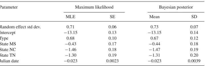
Table 1. Parameter estimates and standard errors for count model parameters obtained with the maximum likeli-hood approach (MLE and SE), together with the corresponding posterior means and standard deviations (SD) from the Bayesian approach.
Parameter Maximum likelihood Bayesian posterior
MLE SE Mean SD
Random effect std dev. 0.71 0.06 0.73 0.07
Intercept −13.15 0.13 −13.15 0.14
Type 0.68 0.10 0.67 0.12
State MS −0.43 0.17 −0.44 0.18
State NC −1.46 0.18 −1.47 0.19
State TN −1.30 0.19 −1.31 0.20
Julian date −0.023 0.0023 −0.023 0.0039
Maximum likelihood estimates of count model parameters and their standard errors were similar to the corresponding posterior means and standard deviations from the Bayesian approach (Table1). The parameter of interest was thetypecovariate. The maximum likeli-hood estimate for this parameter was 0.68 (SE = 0.10) indicating a 97 % increase in covey densities where conservation buffers were present relative to where they were not. This is very close to the Bayesian estimate: the posterior mean for thetypecovariate was 0.67 (SD = 0.12), corresponding to an estimated 95 % increase. (Oedekoven et al. 2014, analysed the full dataset using the Bayesian approach, and estimated that densities were 85 % higher where buffers were present.)
6. DISCUSSION
6.1. OTHEREXAMPLES
Our case study illustrates some of the advantages in adopting a model-based approach. Here, we briefly summarize further examples that illustrate different aspects of the general approach outlined above. We select examples for which there was a clear advantage in adopting a model-based approach.
Buckland et al.(2009) analysed data from a point transect before–after control-impact experiment to assess whether prescribed fire treatments in ponderosa pine forests in the southwestern United States affected densities of two species of warbler. A plot count model was adopted assuming exact distance (Sect.3.1), with an offset that was a function of detectability. A two-stage method was implemented in which detectability was estimated in stage 1, and counts were modelled in stage 2, conditional on estimated detectability. Uncer-tainty in estimated detectability was propagated to stage 2 using a bootstrap. A significant interaction was detected between treatment (control or burning) and year, indicating strong evidence of reduced warbler densities in the year after burning, with moderate evidence of continuing lower densities a year later.
[image:15.496.69.429.108.224.2]States. Many of the sampled sites were in common between the bunting survey and the bobwhite survey of our case study, although the bunting survey was carried out in the breed-ing season, while the bobwhite survey was conducted in the fall. Further, detected buntbreed-ings were assigned to distance intervals, while exact distances were measured for the bobwhites. For the buntings, a plot abundance model for interval distance data was adopted, which is equivalent to a plot count model (Sect.3.2). Thus the approach of Sect.3.1was adopted, and maximum likelihood methods were used to fit the model. The detection function was stratified bystateand the count model included covariates together with a random effect for site. The treatment effect was highly significant, with densities 35 % higher on buffered fields than on control fields.
In this paper, we only superficially address full spatial models for distance sampling. Key papers in this area are Högmander (1991),Hedley and Buckland(2004) andJohnson et al.(2010).Miller et al.(2013) explored how the density of pantropical spotted dolphins varies through a study region in the Gulf of Mexico. Shipboard line transect surveys were carried out, during which sightings and environmental covariates were recorded. In an online appendix, they provide a worked example of how to fit a density surface, based on the methods ofHedley and Buckland(2004). In the case of the spotted dolphins, they found that densities were very variable, and they were able to identify ‘hotspots’.
6.2. GENERALDISCUSSION
ACKNOWLEDGEMENTS
CSO was part-funded by EPSRC/NERC Grant EP/1000917/1. The national CP33 monitoring program was coordinated and delivered by the Department of Wildlife, Fisheries, and Aquaculture and the Forest and Wildlife Research Center, Mississippi State University. The national CP33 monitoring program was funded by the Multistate Conservation Grant Program (Grants MS M-1-T, MS M-2-R), a program supported with funds from the Wildlife and Sport Fish Restoration Program and jointly managed by the Association of Fish and Wildlife Agencies, U.S. Fish and Wildlife Service, USDA-Farm Service Agency and USDA-Natural Resources Conservation Service-Conservation Effects Assessment Project. We thank two anonymous reviewers, whose comments have led to a much improved paper.
Open Access This article is distributed under the terms of the Creative Commons Attribution 4.0 International License (http://creativecommons.org/licenses/by/4.0/), which permits unrestricted use, distribution, and reproduc-tion in any medium, provided you give appropriate credit to the original author(s) and the source, provide a link to the Creative Commons license, and indicate if changes were made.
[Received February 2015. Accepted August 2015.]
REFERENCES
Borchers DL, Buckland ST, Zucchini W (2002) Estimating Animal Abundance: Closed Populations. Springer Verlag, London.
Borchers DL, Burnham KP (2004) General formulation for distance sampling. In: Buckland ST, Anderson DR, Burnham KP, Laake JL, Borchers DL, Thomas L (eds) Advanced Distance Sampling. Oxford University Press, Oxford, pp 6–30
Borchers D, Laake J, Southwell C, Paxton C (2006) Accommodating unmodeled heterogeneity in double-observer distance sampling surveys. Biometrics 62:372–378
Borchers D, Marques T, Gunnlaugsson T, Jupp P (2010) Estimating distance sampling detection functions when distances are measured with errors. Journal of Agricultural, Biological, and Environmental Statistics 15:346– 361
Buckland ST, Anderson DR, Burnham KP, Laake JL, Borchers DL, Thomas L (2001) Introduction to Distance Sampling: Estimating Abundance of Biological Populations. Oxford University Press, Oxford.
Buckland ST, Laake JL, Borchers DL (2010) Double-observer line transect methods: levels of independence. Biometrics 66:169–177
Buckland ST, Russell RE, Dickson BG, Saab VA, Gorman DN, Block WM (2009) Analysing designed experiments in distance sampling. Journal of Agricultural, Biological, and Environmental Statistics 14:432–442
Fewster RM, Buckland ST (2004) Assessment of distance sampling estimators. In: Buckland ST, Anderson DR, Burnham KP, Laake JL, Borchers DL, Thomas L (eds) Advanced Distance Sampling. Oxford University Press, Oxford, pp 281–306
Hedley SL, Buckland ST (2004) Spatial models for line transect sampling. Journal of Agricultural, Biological, and Environmental Statistics 9:181–199
Högmander H (1991) A random fields approach to transect counts of wildlife populations. Biometrical Journal 33:1013–1023
Johnson DS, Laake JL, Ver Hoef JM (2010) A model-based approach for making ecological inference from distance sampling data. Biometrics 66:310–318
Laake JL, Borchers DL (2004) Methods for incomplete detection at distance zero. In: Buckland ST, Anderson DR, Burnham KP, Laake JL, Borchers DL, Thomas L (eds) Advanced Distance Sampling. Oxford University Press, Oxford, pp 108–189
Marques TA, Buckland ST, Borchers DL, Tosh D, McDonald RA (2010) Point transect sampling along linear features. Biometrics 66:1247–1255
Marques TA, Buckland ST, Bispo R, Howland B (2013) Accounting for animal density gradients using independent information in distance sampling surveys. Statistical Methods and Applications 22:67–80
Melville GJ, Welsh AH (2014) Model-based prediction in ecological surveys including those with incomplete detection. Australian and New Zealand Journal of Statistics 56:257–281
Miller DL, Burt ML, Rexstad EA, Thomas L (2013) Spatial models for distance sampling data: recent developments and future directions. Methods in Ecology and Evolution 4:1001–1010
Oedekoven CS, Buckland ST, Mackenzie ML, Evans KO, Burger LW (2013) Improving distance sampling: account-ing for covariates and non-independency between sampled sites. Journal of Applied Ecology 50:786–793
Oedekoven CS, Buckland ST, Mackenzie ML, King R, Evans KO, Burger LW (2014) Bayesian methods for hierar-chical distance sampling models. Journal of Agricultural, Biological, and Environmental Statistics 19:219–239
Oedekoven CS, Laake JL, Skaug HJ (2015) Distance sampling with a random scale detection function. Environ-mental and Ecological Statistics. doi:10.1007/s10651-015-0316-9
Royle JA, Dawson DK, Bates S (2004) Modeling abundance effects in distance sampling. Ecology 85:1591–1597
Royle JA, Dorazio RM (2008) Hierarchical Modeling and Inference in Ecology: The Analysis of Data from Populations, Metapopulations and Communities. Academic Press, San Diego.
Stoyen D (1982) A remark on the line transect method. Biometrical Journal 24:191–195