PSS and SVC Controller Design using Chaos, PSO and SFL Algorithms to Enhancing the Power System Stability

Energy and Power Engineering, 2011, 3, 87-95

doi:10.4236/epe.2011.32012 Published Online May 2011 (http://www.SciRP.org/journal/epe)

PSS and SVC Controller Design Using Chaos, PSO and

SFL Algorithms to Enhancing the Power System Stability

Saeid Jalilzadeh, Reza Noroozian, Mahdi Sabouri, Saeid Behzadpoor

Electrical Engineering Department, Zanjan University, Zanjan, Iran E-mail:{Jalilzadeh, noroozian, M.Sabouri, S.Behzadpoor}@znu.ac.ir,

Received January 8, 2011; revised March 7, 2011; accepted March 15, 2011

Abstract

In this paper, the Authors present the designing of Power System Stabilizer (PSS) and Static Var Compensa-tor (SVC) based on Chaos, Particle Swarm Optimization (PSO) and Shuffled Frog Leaping (SFL) Algo-rithms has been presented to improve the power system stability. Single Machine Infinite Bus (SMIB) sys-tem with SVC located at the terminal of generator has been considered to evaluate the proposed SVC and PSS controllers. The coefficients of PSS and SVC controller have been optimized by Chaos, PSO and SFL algorithms. Finally the system with proposed controllers is simulated for the special disturbance in input power of generator, and then the dynamic responses of generator have been presented. The simulation results show that the system composed with recommended controller has outstanding operation in fast damping of oscillations of power system and describes an application of Chaos, PSO and SFL algorithms to the problem of designing a Lead-Lag controller used in PSS and SVC in power system.

Keywords:Power System Stabilizer (PSS), Static Var Compensator (SVC), Single Machine Infinite Bus (SMIB), Chaos, Shuffled Frog Leaping (SFL), Particle Swarm Optimization (PSO)

1. Introduction

Power systems experience low frequency oscillations (in the range of 0.1 Hz to 2.5Hz) during and after a large or small disturbance has happened to a system, especially for middle to heavy loading conditions [1]. These oscil-lations may sustain and grow to cause system separation if no adequate damping is available [2]. Power System Stabilizers (PSSs) are the most cost effective devices used to damp low frequency oscillations. For many years, Conventional PSSs (CPSSs) have been widely used in the industry because of their simplicity [3]. To improve the performance of CPSSs, numerous techniques have been proposed for their design, such as using intelligent optimization methods (simulated annealing, genetic al-gorithm, tabu search) [4], fuzzy, neural networks and many other nonlinear control techniques. During some operating conditions, PSS may not produce adequate damping, and other effective alternatives are needed in addition to PSS. Recent development of power electron-ics introduces the use of Flexible AC Transmission Sys-tems (FACTS) controllers in power sysSys-tems [5]. FACTS utilize high power semiconductor devices to control the reactive power flow and thus the active power flow of



controller has been simulated for the special disturbance and the dynamic response of generator has been pre-sented.

2. Model of Proposed System

A synchronous machine with an IEEE type-ST1 excita-tion system connected to an infinite bus through a trans-mission line has been selected to demonstrate the deriva-tion of simplified linear models of power system for dy-namic stability analysis [2,10]. Figure 1 shows the model consists of a generator supplying bulk power to an infinite bus through a transmission line, with an SVC located at its terminal. The equations that describe the generator and excitation system have been represented in following equations:



0 1

    ₍₁₎



m e D



1



       (2)









q fd d d q

E    X X id  do



(3)







fd A ref t pss fd

E  K V  V U E T

A (4)

where, m and e are the input and output powers of

the generator, respectively. M and D are the inertia con-stant and damping coefficient, respectively. 0

 

 is the synchronous speed. δ and ω are the rotor angle and speed, respectively.

where, Eq is the internal voltage. fd is the field

voltage.

E d

 

 is the open circuit field time constant. d and d are the d-axis reactance and the d-axis

transient reactance of the generator, respectively. A

 

K

and A are the gain and time constant of the excitation

system, respectively. ref is the reference voltage. Vt

is the terminal voltage. Also and can be ex-pressed as:

T

V

t

V e

t td t

V V  jV_q

q  q  q  (5)

td q q

V   (6)

tq q d d

V   (7)

e Vtd d Vtq

    (8)

where, Xqis the q-axis reactance of the generator.

 

1 d 2 q bsin 3

C C  V  C  (9)

 

4 d 5 q bcos 6

C  C V  C  (10)

Solving (9) and (10) simultaneously, d and q

expressions can be obtained. 1 until 6 are constant

and b is the infinite bus voltage. The various

parame-ters of the system have been represented in Table 1.

C C V Gen q   SVC Infinitive Bus

Vb < 0

Xe

Re

Vt

[image:2.595.312.534.79.169.2]

Id, Iq

Figure 1. Single machine-infinite bus system model with SVC.

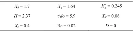
Table 1. System parameters.

Xd = 1.7 Xq = 1.64 d= 0.245

H = 2.37 τ'do = 5.9 XT = 0.08

Xe = 0.4 Re = 0.02 D = 0

3. Static Var Compensator

A Static Var Compensator (or SVC) is an electrical device for providing fast-acting reactive power on high-voltage electricity transmission networks. SVCs are part of the Flexible AC transmission system device family, regulat-ing voltage and enhance the transient stability [11] and provide additional damping to power systems as well [12]. SVC is mainly operated at load side bus and used as replacement for existing voltage control devices [10]. A basic topology of SVC consists of a series capacitor bank C in parallel with a thyristor controlled reactor L, is shown in Figure 2. The SVC can be seen as an adjust-able susceptance which is a function of thyristors firing angle.

4. Power System Linearized Model

A linear dynamic model is obtained by linearizing the nonlinear model round an operating condition (Pe = 1,

Qe = 0.59). The linearized model of power system as

shown in Figure 1 is given as follows:

o   

   (11)

m e D

 



 

    

  (12)





fd d d d

q

do

i

E    q

            

 ₍₁₃₎









fd A ref t pss fd

E K V V U E T

        A SVC (14) 7 8 q

I c  c B

     (15)

9 10 11

d q

I c  c   c BSVC

[image:2.595.310.537.223.277.2] [image:2.595.332.541.569.716.2]

S. JALILZADEH ET AL. ₈₉



d d



c11K9 (21)

C

L

Vt

5. Chaos Algorithm

[image:3.595.120.246.73.341.2]

Chaos is a general phenomenon in non-line system. It can get all the states in the search space by the rules of itself. Moreover, a tiny change of initial values can lead to a big change of the system. The Chaos search can gen-erate the neighbourhoods of near-optimal solutions to maintain solution diversity. It can prevent the search process from becoming premature. The Chaos optimiza-tion method based on Chaos Search is proposed to avoid the local optimal [13]. Chaos variables are usually gen-erated by the well known logistic map. Figure 4 shows the flowchart of Chaos algorithm. The logistic map is a one-dimensional quadratic map defined by following equation:

Figure 2. Basic SVC topology.



1



 



1



i k i k i

    k





(22)

1 2 3

e K K q K svc

  

      B

svc

(17)

where,  is a control parameter and 0i

 

0 

4 1. Despite the apparent simplicity of the equation, the solu-tion exhibits a rich variety of behaviours. For   system (22) generates chaotic evolutions. Its output is like a stochastic output, no value of i is repeated

and the deterministic equation is sensitive to initial con-ditions. Those are the basic characteristics of Chaos. Chaos variable

 

k



 

0

i

 is mapped into the variance ranges of optimisation variables by the following equa-tions [14]:

4 5 6

t q

V K  K   K B

       (18)

1

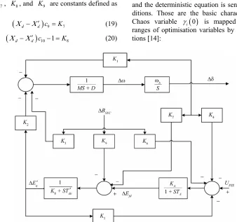
K until K6 are linearization constants. The block

diagram of the linearized power system model is shown in Figure 3. K7, K8, and K9 are constants defined as

follows:



d d



c9 K7

K

(19)



d d



c10 1 8 (20)

Figure 3. Block diagram of the linearized model.

[image:3.595.120.458.385.702.2]

Figure 4. Flowchart of the Chaos algorithm.

 



2

 



i i i i

x k x  k 1 (23)









0.01 , ,

i bi ai xi a bi

    _i (24)

where, x is optimization variable, x is the best ex-periment of variable, and  is the feasible region.

6. PSO Algorithm

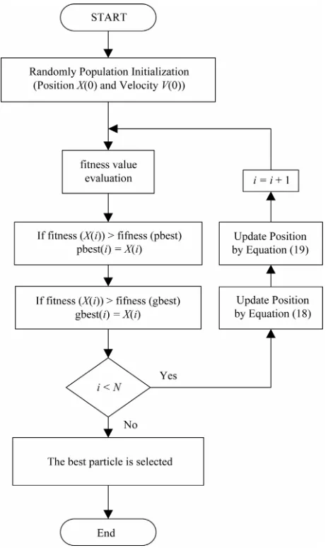
The particle swarm optimization (PSO) algorithm was first proposed by Kennedy and Eberhart [15]. Where is a novel evolutionary algorithm paradigm which imitates the movement of birds flocking or fish schooling looking for food. Each particle has a position and a velocity, rep-resenting the solution to the optimization problem and the search direction in the search space the particle ad-justs the velocity and position according to the best ex-periences which are called the best found by it and

best

p

[image:4.595.63.324.78.641.2]

g found by all its neighbors. In PSO algorithms each particle moves with an adaptable velocity within the re-gions of decision space and retains a memory of the best position it ever encountered. The best position ever at-tained by each particle of the swarm is communicated to all other particles. Figure 5 shows the flowchart of PSO algorithm. The updating equations of the velocity and position are given as follows [16]:

[image:4.595.309.541.317.705.2]

S. JALILZADEH ET AL. ₉₁





1





 

 

 

1 1

2 2

1

i i i i

gi i

v k wv k r c p x k r c p x k

   _  

 

 _  _ (25)



1



 



i i i

x k x k v k (26)

where v is the velocity and x is the position of each par-ticle. 1 and 2 are positive constants referred to as

acceleration constants and must be , usually

1 2 . 1 and 2 are random numbers between 0

and 1, w is the inertia weight, refers to the best posi-tion found by the particle and

c c

r



1 2



4

c c 

2

c c  r

p

g

p refers to the best po-sition found by its neighbors.

7. SFL Algorithm

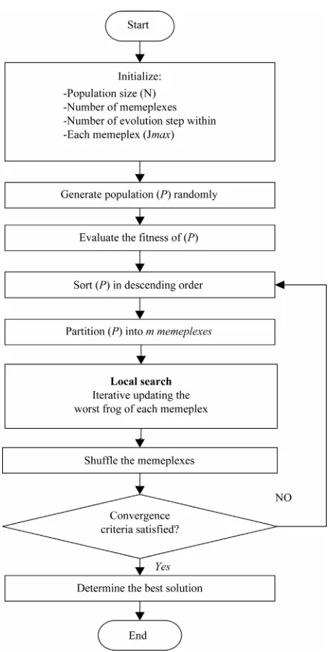
The SFL algorithm is a meta heuristic optimization method that mimic the memetic evolution of a group of frogs when seeking for the location that has the maxi-mum amount of available food. The algorithm contains elements of local search and global information ex-change ([17,18]). The SFL algorithm involves a popula-tion of possible solupopula-tions defined by a set of virtual frogs that is partitioned into subsets referred to as memeplexes. Within each memeplex, the individual frog holds ideas that can be influenced by the ideas of other frogs, and the ideas can evolve through a process of memetic evolution. The SFL algorithm performs simultaneously an inde-pendent local search in each memeplex using a particle swarm optimization like method. To ensure global ex-ploration, after a defined number of memeplex evolution steps (i.e. local search iterations), the virtual frogs are shuffled and reorganized into new memeplexes in a technique similar to that used in the shuffled complex evolution algorithm. In addition, to provide the opportu-nity for random generation of improved information, random virtual frogs are generated and substituted in the population if the local search cannot find better solutions. The local searches and the shuffling processes continue until defined convergence criteria are satisfied. The flowchart of the SFL algorithm is illustrated in Figure 6.

The SFL algorithm is described in details as follows. First, an initial population of N frogs P



X X1, 2, , XN





T

is created randomly. For S-dimensional problems (S variables), the position of a frog in the search space is represented as i 1 2 is

th

i

,



, ,

X  x x 

n x

m N m n

. Afterwards, the frogs are sorted in a descending order according to their fitness. Then, the entire population is divided into memeplexes, each containing frogs (i.e.  



m1



th

), in such a way that the first frog goes to the first meme-plex, the second frog goes to the second memememe-plex, the

frog goes to the memeplex, and the frog goes back to the first memeplex, etc. Let k

th

m _mth

[image:5.595.308.539.71.528.2]

M is the set of frogs in the _kth memeplex, this dividing process

Figure 6. Flowchart of the SFL algorithm.

can be described by the following expression:

 



1 1



, 1



k k m l



.

M  X _{ } P  k n  k m (27)

Within each memeplex, the frogs with the best and the worst fitness are identified as X_b and X_w, respec-tively. Also, the frog with the global best fitness is iden-tified as X_g. During memeplex evolution, the worst frog X_w leaps toward the best frog X_b. According to the original frog leaping rule, the position of the worst frog is updated as follows:



b w



D r X  X (28)





,



max

w w

where, is a random number between 0 and 1; and

max is the maximum allowed change of frog’s position

in one jump.

r D

If this leaping produces a better solution, it replaces the worst frog. Otherwise, the calculations in (28) and (29) are repeated but respect to the global best frog (i.e. re-places Xb). If no improvement becomes possible in this

case, the worst frog is deleted and a new frog is randomly generated to replace it. The calculations continue for a predefined number of memetic evolutionary steps within each memeplex, and then the whole population is mixed together in the shuffling process. The local evolution and global shuffling continue until convergence criteria are satisfied. Figure 6 shows the flowchart of SFL algorithm. Usually, the convergence criteria can be defined as fol-lows:

 The relative change in the fitness of the best frog within a number of consecutive shuffling iterations is less than a pre-specified tolerance;

 The maximum user-specified number shuffling itera-tions is reached.

The SFL algorithm will stop when one of the above criteria is arrived first.

8. Simulation Results

The deviation of speed that obtained from linearization has been selected for inputs of PSS and SVC controller which is shown in Figure 7. As shown in this figure, PSS and SVC have the same Lead-lag controller. The constant values of Figure 7 have been represented in Table 2.

The fitness function used in this paper for Chaos, PSO and SFL algorithms is represented in Equation (30) that

sim is the simulation time, is the deviation of

speed and is the deviation of terminal voltage of generator.

t dw

t

dv

0

10*

sim

t

t

fitness

_

_ dw dv dt_

50

(30)

The deviation of speed ( ) has been multiplied by ten to both section of fitness have the same range. Con-trol parameters and their boundaries are given as follows:

dw

0K (31)

1

0.01T 1 (32)

2

0.01T 1 (33) The convergence rate of the fitness function with num-ber of iterations for SFL, PSO and Chaos algorithms is shown in Figure 8. As shown in Figure 8, the SFL algo-rithm is faster than PSO and Chaos algoalgo-rithm to achieve the optimum coefficients. Table 3 shows the optimized

1

A A

K sT



1

2 1

1 1

w w

sT sT

K

sT sT

  

 

 _  _

1

s s

K sT



1

2 1

1 1

w w

sT sT

K

sT sT

  

 

 _  _

Figure 7. PSS and SVC controller.

Table 2. Constant values.

KA [P.U] TA [P.U] Tw [P.U] Ks [P.U] Ts [P.U]

200 0.02 10 10 0.15

Figure 8. Convergence of SFL, PSO and Chaos algorithms.

Table 3. Optimized values.

SFL PSO Chaos

K 4.42 3.84 3.63

T1 0.164 0.18 0.19

S. JALILZADEH ET AL. ₉₃

(a)

(b)

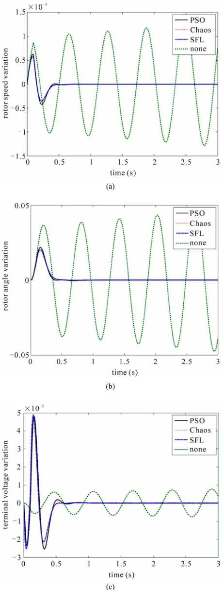
[image:7.595.58.289.77.684.2]

(c)

Figure 9. System dynamic response for a six cycle fault dis-turbance. (a) Rotor speed variation; (b) Rotor angle varia-tion; (c) Terminal voltage variation.

parameters that found by SFL, PSO and Chaos algo-rithms. The final setting of the optimized parameters have been given when the input power of generator has been changed 5% instantaneously and the operating con-dition was Pe = 1 and Qe = 0.59.

Figure 9 shows the system dynamic response for a six cycle fault disturbance for rotor speed variation, rotor angle variation and terminal voltage variation for SFL, PSO and Chaos controllers, also non-controller.

As shown in these figures, it is clear that the perform-ance of PSS and SVC controller has good damping characteristics for low frequency oscillations. However, this improves greatly the power system stability. Also the SFL algorithm has pretty faster behavior in convergence than PSO and Chaos algorithms.

9. Conclusions

In this paper the SMIB system where SVC located at the terminal of generator has been considered. The SVC and PSS have the same controller where their optimized co-efficients have been earned by Chaos, PSO and SFL al-gorithms. In order to show the excellent operation of proposed controller, the input power of generator has been changed 5% instantaneously and the system with proposed controllers has been simulated, then the dy-namic response of generator for rotor speed variation, rotor angle variation and terminal voltage variation have been represented. The effectiveness of the proposed PSS and SVC controllers for improving transient stability performance of a power system are demonstrated under different operating conditions. The simulation results shown that the system composed with proposed control-ler has superior operation in fast damping of oscillations of power system. Also the results show that SFL algo-rithm has pretty faster behavior in convergence than PSO and Chaos algorithms. This procedure can be easily ap-plied to the systems with similar performances.

Humphreys for English editing. All errors are ours.

10. References

[1] S. Sheetekela, K. Folly and O. Malik, “Design and Im-plementation of Power System Stabilizers based on Evo-lutionary Algorithms,” IEEE AFRICON, Nairobi, 23-25 September 2009, pp. 1-6.

doi: 10.1109/AFRCON.2009.5308124

[2] M. A. Abido and Y. L. Abdel-Magid, “Coordinated De-sign of a PSS and an SVC-Based Controller to Enhance Power System Stability,” International Journal of Elec-trical Power and Energy Systems, Vol. 25, No. 9, 2003, pp. 695-704. doi:10.1016/S0142-0615(02)00124-2 [3] A. Phiri and K. A. Folly, “Application of Breeder GA to

Intelli-gence Symposium, St. Louis, 21-23 September 2008, pp. 1-5. doi: 10.1109/SIS.2008.4668328

[4] W. X. Liu, G. K. Venayagamoorthy and D. C. Wunsch II, “Adaptive Neural Network Based Power System Stabi-lizer Design,” Proceedings of the International Joint Conference on Neural Networks, Portland, 20-24 July 2003, pp. 2970-2975. doi: 10.1109/IJCNN.2003.1224043 [5] S. Panda, “Multi-Objective Non-Dominated Shorting

Genetic Algorithm-II for Excitation and TCSC-Based Controller Design,” Journal of Electrical Engineering, Vol. 60, No. 2, 2009, pp. 86-93.

[6] N. G. Hingoran and L. Gyugyi, “Understanding FACTS, Concepts and Technology of Flexible AC Transmission System,” Institute of Electrical and Electronics Engi-neering, Inc., New York, 2000.

[7] N. G. Hingorani, “High Power Electronics and Flexible AC Transmission System,” IEEE Power Engineering re-view,Vol. 8, No. 7, 1988, pp. 3-4.

doi:10.1109/MPER.1988.590799

[8] R. Jayabarathi, M. R. Sindhu, N. Devarajan and T. N. P. Nambiar, “Development of a Laboratory Model of Hy-brid Static Var Compensator,” IEEE Power India Con-ference, Ner Delhi, 2006, p. 5.

doi: 10.1109/POWERI.2006.1632507

[9] P. F. Puleston, S. A. Gonza´lez and F. Valenciaga, “A STATCOM Based Variable Structure Control for Power System Oscillations Damping,” International Journal of Electrical Power and Energy Systems, Vol. 29, No. 3, 2007, pp. 241-250. doi:10.1016/j.ijepes.2006.07.003 [10] Y. P. Wang, D. R. Hur, H. H. Chung, N. R. Watson, J.

Arrillaga and S. S. Matair, “A Genetic Algorithms Aproach to Design Optimal PI Controller for Static Var Compensator,” IEEE International Conferences on Power System Technology, Perth, 2000, pp. 1557-1562. doi: 10.1109/ICPST.2000.898203

[11] S. K. Tso, J. Liang, Q. Y. Zeng, K. L. Lo and X. X. Zhou, “Coordination of TCSC and SVC for Stability Improve-ment of Power Systems,” Proceedings of the Fourth

In-ternational Conference on Advances in Power System Control, Operation and Management, Hong Kong,11-14 November 1997, pp. 371-376. doi: 10.1049/cp:19971862 [12] K. R. Padiyar and R. K. Varma, “Damping Torque

Analysis of Static Var System Controllers,” IEEE Transacions on Power Systems, Vol. 6, No. 2, 1991, pp. 458-465. doi:10.1109/59.76687

[13] S. Wang and B. Meng, “Chaos Particle Swarm Optimiza-tion for Resource AllocaOptimiza-tion Problem,” IEEE Interna-tional Conference on Automation and Logistics, Jinan, 18-21 August 2007, pp. 464-467.

doi: 10.1109/ICAL.2007.4338608

[14] L. Shengsong, W. Min and H. Zhijian, “Hybrid Algo-rithm of Chaos Optimisation and SLP for Optimal Power Flow Problems with Multimodal Characteristic,” IEE Proceedings of Generation, Transmission and Distribu-tion, Vol. 150, No. 5, pp. 543-547.

doi: 10.1049/ip-gtd:20030561

[15] M. Y. Shan, J. Wu and D. N. Peng, “Particle Swarm and Ant Colony Algorithms Hybridized for Multi-Mode Re-source-constrained Project Scheduling Problem with Minimum Time Lag,” IEEE International Conference on Wireless Communications, Networking and Mobile Computing, Shanghai, 21-25 September 2007, pp. 5898- 5902. doi: 10.1109/WICOM.2007.1446

[16] L. Zhao and Y. Yang, “PSO-Based Single Multiplicative Neuron Model for Time Series Prediction,” International Journal of Expert Systems with Applications, Vol. 6, No. 2, 2009, pp. 2805-2812.

doi: 10.1016/j.eswa.2008.01.061

[17] M. Morari and E. Zufiriou, “Robust Process Control,” Prentice-Hall, Inc., Englewood Cliffs, 1987.

S. JALILZADEH ET AL. ₉₅

Notation

m

Ρ Ρ

The input power of the generator

e The output power of the generator

M The inertia constant

D The damping coefficient

0

 The synchronous speed

 The rotor angle

 The rotor speed

q

E The internal voltage

fd

'd

E The field voltage

 The open circuit field time constant

d

 The d-axis reactance of the generator

q

X The q-axis reactance of the generator

d

X The d-axis transient reactance of the generator

A

K The gain of the excitation system

A

V

T The time constant of the excitation system

ref

V

The reference voltage

t

C

The terminal voltage

1C

V 6

6

The constants

b The infinite bus voltage 1

K K The linearization constants

7 9

K K ,

The constants defined in (19), (20), (21)

i

  The basic characteristics of Chaos

x The optimization variable of Chaos

x _{The best experiment of variable of Chaos}  The feasible region of Chaos

V The velocity of PSO

X The position of each particle of PSO

1and

c c2

2

The positive constants referred to as accelera-tion

1and

v v

W

The random numbers between 0 and 1 in PSO The inertia weight in PSO

and g

p p The best position found by the particle and the best position in PSO, respectively

b

X The frog with the best fitness of SFL

w

X The frog with the worst fitness of SFL

g

X The frog with the global best fitness of SFL

r A random number between 0 and 1 in SFL

max

D The maximum allowed change of frog’s posi-tion in one jump in SFL

sim

t dw

The simulation time The deviation of speed

t