Advanced Semi Active Resetable Devices and Device Modeling Including Non Linearities

Advanced Semi-Active Resetable Devices and

Device Modeling Including Non-Linearities

J. Geoffrey Chase* Geoffrey W. Rodgers* Kerry J. Mulligan* and Rodney B. Elliott* *Dept of Mechanical Engineering, University of Canterbury, Christchurch, New Zealand

E-mail: [email protected]

Abstract

Resetable devices are a novel semi-active approach to managing structural response energy. Recently developed devices allow independent control of each chamber enabling unique approaches to sculpting the structural hysteresis loops and behaviour. This paper creates a non-linear model of experimental prototypes that is fully generalisable, and does so in a step-by-step fashion adding each non-linear affect individually. Non-linearities that can significantly affect performance, including valve size, mass flow rate and friction are characterised experimentally and modeled. The results are validated against experimental data for cases of all forms of device control, as well as for several experimental cases utilizing external pressurized sources to enhance the force capacity. Force capacity, using a pressurised reservoir and/or accumulator increased force capacity of these devices from 100-600%, increasing the potential of these designs and approach to seismic energy dissipation. Final model results have less than 5% error compared to nonlinear experimental data. There is a strong correlation between the fundamental nonlinear dynamics modelled and the experimental results, validating the overall model and approach. The overall results and approach are fully general for application to the design or analysis of similar device systems.

Key words: Seismic Response, Semi-Active Control, Structural Dynamics, Resetable Devices

(1 blank line)

1. Introduction

This paper develops a non-linear analytical model to describe the dynamic and transient force-displacement behaviour of resetable devices that utilize air as the working fluid. However, the models may be fully and directly generalised to other working fluids. Kajima Corp. has 1-4 control law devices based on Jabbari et al [1]. The initial independently controlled chamber device design examined here is detailed by Chase et al [2].

it is possible to use different working fluids other than air. Air was used in this case for simplicity as the vented and reservoir fluid volumes are the surrounding atmosphere, eliminating the need for extra fluid management devices and system.

In this research, a progression of models of the device behaviour are developed that capture the device dynamics. Each successive model more accurately captures observed device dynamics. The models are validated by comparing the model prediction and experimental results for a variety of device control laws and input motions. Finally, a next generation resetable devices is introduced that offers enhanced force capacity to improve the range of potential applications. They also offer further enhanced adaptability in control laws, the resulting force-displacement behaviour, and thus enhanced ability to sculpt structural hysteretic response [2-5].

2. Model Development:

2.1 Linear Model:

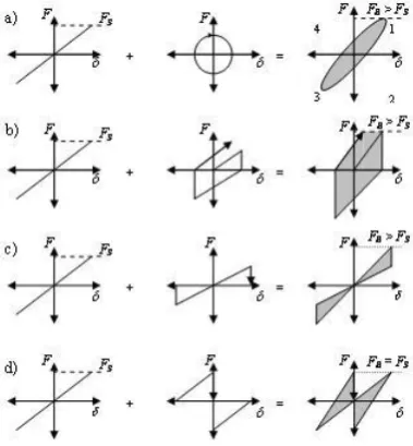
The simplest device model is a linear spring where the force produced is thus a constant multiple of the piston displacement from a prior reset [1, 2, 5]. This constant is the nominal device stiffness and is dependent on the initial chamber volume and rate of change of the chamber volume with piston displacement, which are functions of the device design dimensions. Figure 1 shows force-displacement diagrams using a linear model for the fundamental 3 device control laws [5], as well as a viscous damper. The prototype devices constructed for this research were designed around a nominal stiffness of 250kN/m and 590kN/m respectively. In this research, the stiffness is altered by simply changing the piston design and chamber length and thus modifying the initial chamber volumes [2, 3].

Figure 1: Linear hysteretic response of resetable device. Device resets result in zero force from a peak value and occur at different locations in a sinusoidal response in this schematic.

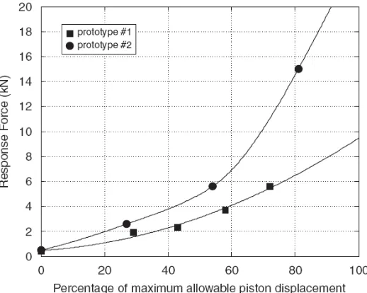
Figure 2: Peak force versus the percentage of maximum allowable piston displacement for both

prototypes. Both devices have a non-linear response with the second prototype clearly having a higher stiffness and greater non-linearity at piston displacements above 60% of the maximum displacement.

2.2 Ideal Gas Law Model:

The linear model can be superseded with a more realistic, still simple model based on ideal gas laws. The device force response for a change in chamber volume is dependent on the active chamber pressure, where the active chamber is the chamber decreasing in volume due to piston (device input) motion. The pressure in each chamber is thus defined:

 ) ( =

2 1 1 2

V V p

p (1)

Where p1 and p2 are the pressures before and after piston displacement, V1 and V2 are the volumes of the active chamber before and after piston displacement, and  is the ratio of specific heats. The resulting force, F, produced is defined:

A p p

F=( c1 c2) (2)

where pC1 and pC2 are the pressures in each chamber, and A is the piston area.

The ideal model assumes an instantaneous energy (pressure) release at reset. It also assumes zero force developed when the chambers are open (no friction), as well as exactly symmetric behaviour. Instantaneous energy release dictates that the response force returns to zero immediately after a valve is opened. Symmetric behaviour requires the central piston position to be perfectly assigned.

This ideal gas based model still captures most of the device behaviour over all frequencies and amplitudes of input motion, as seen in Figure 3. However, error and further nonlinearity is observed. These differences can have a significant effect on the device response, as seen in the 3.0Hz response. Hence, physical contributions including friction in the device and non-linear air flow dynamics through the valves need to be added to produce an accurate, fully representational model of these devices. In addition, control system dynamics that operate the device valves can also contribute to the overall behaviour of the devices and should thus be accounted for.

The shape of the device force-displacement response is determined by the device control law. A variety of control laws can be implemented [2-6]. However, fundamental

Figure 3: Experimental and model device response under 1-3 control for 10mm sinusoidal piston motion at 0.1, 0.5 and 1Hz (LEFT); and for the 2-4 control law (RIGHT). The model prediction captures most of the experimental behaviour.

2.3 Enhanced Nonlinear Model - Friction:

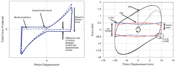
The most obvious difference between the experimental and ideal model results is the force discrepancy after pressure release. The ideal model assumes a return to zero force on reset, but experimentally, the device force returns to a non-zero value due to friction inside the device, as seen in Figure 4. The amount of friction is readily determined by measuring the device response to piston displacements with both valves open, which limits the force generated by chamber pressure. The rigth plot of Figure 4 shows the device response to sinusoidal motion with 10 mm displacement at 0.1, 1.0 and 3.0Hz. From these figures, the friction contribution is identified as 0.4-0.5kN, from the the 0.1 and 1.0Hz motions.

Figure 4: Experimental result and ideal model prediction showing the contribution of friction (LEFT) and open valve experiments to determine friction force contribution (RIGHT).

force, and for slower motions it is effectively the only force generated. This approach for determining the static friction parameter is readily generalised to other working fluids.

The friction force was thus incorporated into the ideal model by resetting the device force to the friction level, rather than zero. The sign of the friction force is dependent on the direction of piston motion. Thus, when the piston changes direction the total change in force is twice the friction force value, as shown in Figure 4. The additional force resulting from 'insufficient' air flow through the valves for the high frequency piston motion in Figure 4 is accounted for later using an energy release rate model.

2.4 Enhanced Nonlinear Model – Air Flow Release Rate Model:

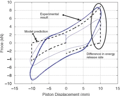
The ideal model assumes that when the valves open the pressure instantly equalises with the pressure of the external fluid reservoir yielding an instant drop in force to friction levels and a perfectly vertical line on a force-displacement plot. However, there is always a finite air flow rate through any valve. In this research, the time required for sufficient flow to occur and for pressure to equalise is significant compared to the device motion. Hence, there is some time lapse between the valves opening and the pressure equalising, resulting in a more diagonal line or gradient on the force-displacement plot, as shown in Figure 5.

Figure 5: Experimental result and model prediction for 10mm, 2Hz sinusoidal input motion showing difference in energy release rates, where the model assumes an instantaneous energy release.

The air flow rate through the valves is dependent on the size of the valve opening and the pressure difference between the air inside the chamber and the external fluid reservoir. In general, the open valve can be assumed to be a circular orifice. The flow through the orifice is determined to be choked or non-choked depending on the pressure gradient across the orifice. Non-choked flow rates dependent on the pressure gradient between the high pressure and low pressure zones on each side of an orifice. Choked flow is the limiting rate of flow depending on the size and type of an orifice. For a circular orifice, the flow is choked if the following inequality is valid [7].

1 ) 2 1 (       a s p

p ₍₃₎

where ps is the upstream pressure, pa is the down stream pressure, atmospheric for most cases and 1.4 is the ratio of specific heats, in this case for air.

The resulting mass flow rate,

m



2 2 1 ) 1 2 ( =       RT kM CAp

and: ] ) ( ) )[( 1 ( 2 = 1 2      _   s a s a s p p p p RT M CAp

m (flow not choked) (5)

where C is the orifice coefficient, A is the orifice area, M is the molecular weight, R is the universal gas law constant, and ps, pa and  are as previously defined.

The ideal model uses the air pressure inside each chamber as the basic dynamic parameters. However, with the added complexity of incorporating the air flow rate through the valves the air mass in each chamber is more representative and intuitive. Using the air mass as the base parameter readily accommodates using the air mass flow rate through the valves in the model.

The mass flow rate is calculated using Equations 4 and 5, and multiplied by t to obtain the total average mass change, due to flow through the valve, for each time step. Using the mass of air ensures the model obeys the fundamental conservation laws by not allowing the mass to increase beyond the equilibrium mass, defined by the chamber volume at atmospheric pressure with the valve open. Hence, the model based on working fluid mass (m) accounts for the reduction in air mass with a decrease in volume, an effect that was not specifically accounted for in the ideal pressure model.

The finite air flow rate through the valves is particularly noticeable for high frequency piston motion, as seen in the right plots of Figures 3-4. It is particularly evident in the device response to the 2-4 control law due to the fact that its device reset command occurs at peak velocity when the piston crosses zero. For high frequency motion, the length of time required for the air mass to decrease to the equilibrium mass can become a significant percentage of the piston cycle time. Therefore, the mass reaches equilibrium after the piston has moved through a potentially large amount of the subsequent cycle. The result is a curved reset line on the force-displacement plot, as shown in Figure 6 for a 2-4 control law, resulting in a force displacement shape that is almost diamond-shaped.

Figure 6: Experimental result to 15mm, 1Hz sinusoidal motion with the 2-4 control law. The chamber

volume is still decreasing after the valve is opened resulting in an apparent delay between valve actuation and the force decreasing

dynamics appears as a delay in the force reduction until a measurable displacement after the zero position in some cases. This behaviour is also evident in Figure 6.

Finally, the air flow rate into the device via open valves is modelled using the same mass flow rate equations. For low frequency piston motion, the air mass inside the open chamber will be the equilibrium mass as the rate of air flow in through the valves exceeds the required change air mass to maintain the equilibrium mass. However, for high frequency piston motion the mass flow rate through the valves may not be sufficient to maintain the equilibrium mass inside the open chamber. Hence, the pressure inside the chamber falls below equilibrium pressure for the chamber volume, and at times below the external fluid reservoir or atmospheric pressure. This lower pressure yields a greater pressure gradient between chambers and thus a slightly greater overall force is produced in these cases. Overall, using these mass flow equations all these effects are included in the model.

2.5 Enhanced Nonlinear Model – Valve Control Delays:

To complete the enhanced model, the delay between the valve solenoid being commanded to switch states and air beginning to flow through the opened valve is included. This delay is physically comprised of the delay between the command signal being sent to the valve and the solenoid receiving the signal, as well as the time taken for the valves to operate once the solenoid has received the command signal. The total solenoid command and valve delay is modelled as a fixed hold period on the state of the valve after the model has detected that a switch command has occurred.

The delay, as measured from experiments, is not constant and the time taken for the valves to operate after receiving the signal to switch depends at least partially on the pressure inside the chamber at that time. An average experimental value of 0.01 seconds was used in the model and is a good compromise between incorporating the delay effect simply and undue complexity. Typically, the delay value appears insignificant. However, at high frequency, the delay forms a noticeable part of the device response, as seen in Figure 7. Specifically, the 0.01s delay at peak velocity (zero displacement) for the 2-4 device control law results in a 1.25 to 1.90mm delay for 10 to 15mm amplitude sinusoidal displacement motions at 2Hz.

Figure 7: Modelled and experimental response to 2.0Hz motion. Note the delay between the piston

passing the 0 position and the change in response slope indicating when the valve actually closed.

2.5 Model Summary and Procedure:

describe the device dimensions and working fluid characteristics. The dynamic inputs are dependent on the input, or relative, motion of the piston as well as the valve control depending on the control law implemented. The calculation section determines the air mass in each chamber depending on the given inputs. Finally, the results for each time step are generated. These results are the pressure in chamber depending on the air mass and chamber volume and the reaction force obtained from the differential pressure in the two chambers. The model can be run at any reasonable time step size, where typically the same time step used in controlling experimental systems would be used.

Figure 8: Flowchart showing enhanced nonlinear model calculation procedure.

3. Model Validation:

The model was validated by comparison with experimental results from two experimental device configurations:

• A device working from atmospheric (reservoir) pressure

• A device working from greater than atmospheric (reservoir) pressure

The final model is compared to experimental device responses within the input motion ranges of interest in Figure 9.

Figure 9 compares the experimental and modeled results for various input motions and control laws. The ability of the nonlinear model to capture the device dynamics is evident. The comparison in Figure 11d shows a slight discrepancy due to the high frequency input motion. At this high frequency small differences between the modeled valve flow dynamics or friction, and the actual flow dynamics or friction assumptions are amplified.

Still the result in Figure 11d is quite close for a device operation regime that would not be desirable by design. Thus, devices likely to be subject to such higher frequencies would require greater valve diameters (or numbers of valves) to recapture the 2-4 device control law shape of Figure 11c. Thus, what Figure 11d shows most clearly is the robustness of the model and dynamics developed in its ability to capture such a highly non-linear case.

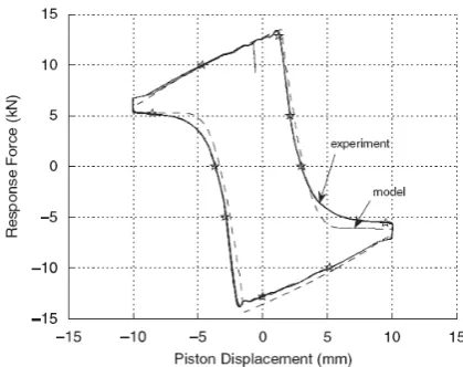
The final model is also highly adaptable to capturing variable device configurations and different external conditions, such as high pressure external reservoirs. Figure 10 shows the experimental and modelled results for the 2-4 control case with a piston displacement of 10mm at 0.5Hz, and the air supply at 2.0 additional atmospheres. The maximum forces and overall experimental force-displacement loop are well predicted by the model including the energy release slope. Valve specific model parameters can also be readily altered to account for different valve types, valve control or valve architectures.

Figure 10: Force-displacement response of the device comparing experimental and modeled data for a 10mm and 0.5Hz input. Note the model accurately captures the device response.

4. Conclusions:

A non-linear dynamic model of unique semi-active resetable devices is derived and validated based on experimental data. The model incorporates all experimentally observed nonlinear device dynamics. Using the device design dimensions and knowledge of the valve operation, a realistic and highly accurate prediction of device response can be obtained. The important attributes incorporated in the final non-linear model:

 Ideal gas law behaviour

 Friction between moving parts

 Air flow rates into and out of the device

 Valve operation delay

 Calculation of dynamic variable air mass in chamber

 Other working fluids

 Additional external dynamics such as those from reservoirs or pressurising pumps

 Different valve types, valve control or valve numbers

 Any other likely effects observed

Finally, such non-linear models may be used to better design semi-active systems or experiments, as well as for optimizing those devices to a given application requirement.

References:

[1] F. Jabbari and J. E. Bobrow, "Vibration Suppression with a Resetable Device," ASCE Journal of Engineering Mechanics, vol. 128(9), pp. 916-924, 2002.

[2] J. G. Chase, K. J. Mulligan, A. Gue, T. Alnot, G. Rodgers, J. B. Mander, R. Elliott, B. Deam, L. Cleeve, and D. Heaton, "Re-shaping hysteretic behaviour using semi-active resettable device dampers," Engineering Structures, vol. 28, pp. 1418-1429, Aug 2006. [3] K. J. Mulligan, "Experimental and analytical studies of semi-active and passive

structural control of buildings," in Mechanical Engineering. vol. PhD Christchurch: University of Canterbury, 2007, p. 260.

[4] K. Mulligan, J. Chase, J. Mander, G. Rodgers, R. Elliott, R. Franco-Anaya, and A. Carr, "Experimental Validation of Semi-active Resetable Actuators in a 1/5th Scale Test," Earthquake Engineering & Structural Dynamics (EESD), vol. 38, pp. 517-536, 2009.

[5] G. W. Rodgers, J. B. Mander, J. G. Chase, K. J. Mulligan, B. L. Deam, and A. Carr, "Re-shaping hysteretic behaviour - spectral analysis and design equations for semi-active structures," Earthquake Engineering & Structural Dynamics, vol. 36, pp. 77-100, Jan 2007.

[6] K. J. Mulligan, J. G. Chase, A. Gue, T. Alnot, G. W. Rodgers, J. B. Mander, R. B. Elliott, B. L. Deam, L. Cleeve, and D. Heaton, "Large Scale Resetable Devices for Multi-Level Seismic Hazard Mitigation of Structures," Proc. 9th International Conference on Structural Safety and Reliability (ICOSSAR 2005), Rome, Italy, June 19-22., 2005.