Wavelet Bases Made of Piecewise Polynomial Functions: Theory and Applications

(1)

doi:10.4236/am.2011.22022 Published Online February 2011 (http://www.SciRP.org/journal/am)

Wavelet Bases Made of Piecewise Polynomial Functions:

Theory and Applications

*

Lorella Fatone1, Maria Cristina Recchioni2, Francesco Zirilli3 1

Dipartimento di Matematica e Informatica, Università di Camerino, Camerino, Italy

2

Dipartimento di Scienze Sociali “D. Serrani”, Università Politecnica delle Marche, Ancona, Italy

3

Dipartimento di Matematica “G. Castelnuovo”, Università di Roma “La Sapienza”, Roma, Italy E-mail: [email protected], [email protected], [email protected]

Received October 8, 2010; revised November 26, 2010; accepted December 1, 2010

Abstract

We present wavelet bases made of piecewise (low degree) polynomial functions with an (arbitrary) assigned number of vanishing moments. We study some of the properties of these wavelet bases; in particular we consider their use in the approximation of functions and in numerical quadrature. We focus on two applications: integral kernel sparsification and digital image compression and reconstruction. In these application areas the use of these wavelet bases gives very satisfactory results.

Keywords:Approximation Theory, Wavelet Bases, Kernel Sparsification, Image Compression

1. Introduction

In the last few decades wavelets and wavelets techniques have generated much interest, both in mathematical analysis as well as in signal processing and in many other application fields. In mathematical analysis wavelet bases, whose elements have good localization properties both in the spatial and in the frequency domains, are very useful since, for example, they consent to approximate functions using translates and dilates of one or of several given functions. In signal processing, wavelets were initially used in the context of subband coding and of quadrature mirror filters, but later they have been used in a variety of applications, including computer vision, image processing and image compression. The link between the mathematical analysis and signal processing approaches to the study of wavelets was given by Coif-man, Mallat and Meyer (see [1-6]) with the introduction of multiresolution analysis and of the fast wavelet transform, and by Daubechies (see [7]) with the introduction of orthonormal bases of compactly supported wavelets.

Let A be an open subset of a real Euclidean space

and let L2

 

A be the Hilbert space of the square inte-

grable (with respect to Lebesgue measure) real func-

tions defined on A. In this paper when A is a suffici-

ently simple set (i.e. a parallelepiped in the examples

considered), starting from the notion of multiresolution

analysis, we construct wavelet bases of L2

 

A with an

(arbitrary) assigned number of vanishing moments. The main feature of these wavelet bases is that they are made of piecewise polynomial functions of compact support; moreover the polynomials used are of low degree and generate bases with an arbitrarily high assigned number of vanishing moments. This fact makes possible to perform very efficiently some of the most common computations, such as, for example, differentiation and integration. However the lack of regularity of the piecewise polynomial functions used can create undesirable effects in the points where the discontinuities occur when, for example, continuous functions are approximated with discontinuous functions. Note that the wavelet bases studied here, in general, make use of more than one wavelet mother function. Thanks to these properties these wavelet bases in several applications can outperform in actual computations the classical wavelet bases and, for example, in this paper we show that they have very good approximation and compression properties. The numerical results of Se- ction 4 corroborate these statements both from the qua- litative and the quantitative point of view.

The wavelet bases introduced generalize the classical Haar’s basis, that has only one vanishing moment and is made of piecewise constant functions (see, for example, [8]), and are a simple variation of the multi-wavelets *

(2)

bases introduced by Alpert in [9,10]. The results reported here extend those reported in [11,12] and aim to show not only the theoretical relevance of these wavelet bases (also shown, for example, in [9,10,13,14]) but also their effective applicability in real problems. In particular in this paper we study some properties of the wavelet bases considered and the advantages of using some of them in simple circumstances. In fact the orthogonality of the

wavelets to the polynomials up to a given degree (i.e. the

vanishing moments property) plays a crucial role in producing “sparsity” in the representation using these wavelet bases of functions, integral kernels, images and so on. These wavelet bases as the wavelet bases used previously have good localization properties both in the spatial and in the frequency domains and can be used fruit- fully in several classical problems of functional analysis. In particular we focus on the representation of a function in the wavelet bases and we present some ad hoc quadrature formulae that can be used to compute efficiently the coefficients of the wavelet expansion of a function.

We consider also the use of these wavelet bases in some applications, initially we focus on integral kernel sparsification. This is a relevant task, see for example [10,15], since it makes possible, among other things, the approximation of some integral operators with sparse matrices allowing the approximation and the solution of the corresponding integral equations in very high dimensional subspaces at an affordable computational cost. In [11,12,16], for example, we exploit this property to solve some time dependent acoustic obstacle scattering problems involving realistic objects hit by waves of small wavelength when compared to the dimension of the objects. Let us note that these scattering problems are trans- lated mathematically in problems for the wave equation and that they are numerically challenging, moreover thanks to the use of the wavelet bases, when boundary integral methods or some of their variations are used, they can be approximated by sparse systems of linear

equations in very high dimensional spaces (i.e. linear

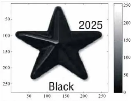
systems with millions of unknowns and equations). Later on we focus on another important application of wavelets: digital image compression and reconstruction. In this framework, the basic idea is to distinguish between relevant and less relevant parts of the image details dis- regarding, if necessary, the second ones. In particular we proceed as follows: a digital image is represented as a sequence of wavelet coefficients (wavelet transform of the original image), a simple truncation procedure puts to

zero some of the calculated wavelet coefficients (i.e.

those that are smaller than a given threshold in absolute value) and keeps the remaining ones unaltered (com-

pression). The truncation procedure is performed in such

a way that the reconstructed image (i.e. the image ob-

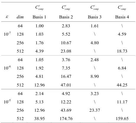
tained acting with the inverse wavelet transform on the truncated sequence of wavelet coefficients) is of quality comparable with the quality of the original image, but the amount of data needed to store the compressed image is much smaller than the amount of data needed to store the original image. We present some interesting numerical results in wavelet-based image compression and reconstruction. Moreover we define a compression coefficient to evaluate the performance of the compression procedure and we study the behaviour of the compression coefficients on some test problems, in particular we show that the compression coefficients increase when the number of vanishing moments of the wavelet basis used increases. This property can be exploited in several practical applications.

The paper is organized as follows. In Section 2 using a multiresolution approach we present the wavelet bases. In Section 3 some mathematical properties of the wavelet bases introduced are discussed and some applications of these bases to function approximation are shown. Fur- thermore some quadrature formulae that exploit the bases properties are presented. In Section 4 applications of the wavelet bases introduced to kernel sparsification and image compression are shown. In particular in Subsection 4.1 we study some interesting properties of the bases considered and we present some results about integral kernel sparsification. In Subsection 4.2 we focus on applications of the wavelet bases to image coding and compression showing some interesting numerical results. Fi- nally in the Appendix we give the wavelet mother functions necessary to construct the wavelet bases employed in the numerical experience presented in Section 4. To build these mother functions we have used the Symbolic Math Toolbox of MATLAB. The website http://www. econ.univpm.it/recchioni/scattering/w17 contains auxili- ary material and animations that help the understanding of the results presented in this paper and makes available to the interested users the software programs used to generate the wavelet mother functions of the wavelet bases used to produce the numerical results presented. A more general reference to the work of the authors and of their coworkers in acoustic and electromagnetic scattering where the wavelet bases introduced have been widely used is the website http://www.econ.univpm.it/recchioni /scattering.

2. Multiresolution Analysis and Wavelets

(3)

Mallat [1,2], Meyer [3-5] and Coifman and Meyer [6] to construct wavelet bases. Let us begin introducing some

notation. Let Rbe the set of real numbers, given a posi-

tive integer s let Rs be the s-dimensional real Eucli-

dean space, and let =



1, 2, ,



T s s

x x x  x R be a gene-

ric vector where the superscript T means transposed.

Let ( , )  and  denote the Euclidean scalar product and the corresponding Euclidean vector norm respectively.

For simplicity we restrict our analysis to the interval

(0,1). More precisely, we choose A= 0,1

 

R. Let

 





2

0,1

L be the Hilbert space of square integrable

(with respect to Lebesgue measure) real functions defined on the interval (0,1). We want to construct ortho-

normal wavelet bases of L2



 

0,1



via a multiresolu-

tion method similar to the methods used in [9,1-6]. Note that using the ideas suggested in [13,14] it is possible to generalize the work presented here to rather general do-

mains A in dimension greater or equal to one.

Given an integer M1, we consider the following

decomposition of 2



 



0,1

L :

 







 





 



2

0,1 = M 0,1 M 0,1 ,

L P V (1)

where  denotes the direct sum of two orthogonal

closed subspaces PM



 

0,1



and VM



 

0,1



of

 





2

0,1

L . In other words, the vector space generated by

the union of M



 

0,1



P and M



 

0,1



V is 2



 



0,1

L

and we have:

   



 





 



1

0 = 0, 0,1 , 0,1 .

M M

dx f x g x  f P gV



(2)

We take _PM



 

0,1



to be the space of the poly-

nomials of degree smaller than M defined on (0,1) and

we consider a basis of M



 

0,1



P made of M polyno-

mials orthogonal in the interval (0,1) with respect to the weight function w x

 

= 1, x

 

0,1 , having _L2

-norm equal to one. For example we can choose as basis of

 



0,1



M

P the first M Legendre orthonormal polyno-

mials defined on (0,1) and we refer to them asL xq( ),

(0,1),

x q= 0,1,,M1.

To construct a basis of VM



 

0,1



we use the ideas

behind the multiresolution analysis. Let us begin defining

the so called “wavelet mother functions”. Let N2 be

an integer and let





1

1 2 1

= , , , T

N N

N R

    

 

 be a

vector whose elements _i

 

0,1 , i= 1, 2,,N1, are such that ηi<ηi1, i= 1, 2,,N2. Given the integers

J, M, N, such that J1, 1,M 2,N we define the

following piecewise polynomial functions on (0,1):

1 1, , ,

1 , , 1, , ,

1 , , ,

( ), (0, ),

( ) = ( ), [ , ), = 1, 2, , 2,

( ), [ ,1),

M N j N

M M

N N i i

j N i j N M

N N

N j N

p x x

x p x x i N

p x x

            _           

= 1, 2, , ,

j  J (3)

where

 

₌₀1



 



, , , = , , , , , 0,1 ,

M

M l M

N l N

i j N l i j M N

p x q x P

 







= 1, 2, , ,

i  N j= 1, 2,, ,J are polynomials of degree

smaller than M to be determined. The functions

, , , M

N j N

 j= 1, 2,, ,J defined in (3) will be used

as “wavelet mother functions”. In fact through them we generate the elements of a wavelet family via the multiresolution analysis.

For simplicity let us choose i = /i N, i= 1, 2,,

1

N . We note that results analogous to the ones

obtained here with this choice can be derived for the general choice of i, = 1, 2,i ,N1, at the price of having more involved formulae.

Let us define the functions:

 













 





2 , , , , , , ,

= _, ₁ _,

0, 0,1 \ , 1 ,

m M m N j N M m m N j m N

m m

N N x

x _x _N _N

x N N

     _ _             _ _   _ _ 

= 0,1, ,_Nm 1,_m= 0,1, , = 1, 2,_j , ,_J

     (4)

whose supports are the intervals



Nm,



1



Nm



 

0,1 ,

  = 0,1,,Nm1, m= 0,1,. Moreover we

define the set of functions



 



, , 0,1 M

N N J

W _ as follows:

 







 



, , , , , ,

0,1 = , 0,1 , = 0,1, , 1,

, (0,1), = 1, 2, , ,

= 0,1, , = 0,1, , 1 ,

M

N q

N J M

N j m N

m

W L x x q M

x x j J

m N              (5)

where Lq

 

x , q= 0,1,,M1, and _, _, ( ),

M N j N x



 

0,1 ,

x j= 1, 2,, ,J are the functions defined above when we choose N = 1



N, 2 N, 3 N,,



N1



N



T.

We want to choose J, M , N, and the coefficients

of the polynomials that constitute the functions

, , , M

N j N

 j= 1, 2,, ,J defined in (3), that is the

coefficients

, , , , , N l i j M N

q

 , l= 0,1,,M1, of , , , M

N i j N

p

 ,

= 1, 2, ,

j  J, = 1, 2,i ,N, in order to guarantee that

the set



 



, , 0,1 M

N N J

W _ defined in (5) is an orthonormal

(4)

satisfy some constraints specified later imposing the following conditions to the wavelet mother functions (3):

i) the functions

, , , M

N j N

 j= 1, 2,, ,J have the

first M moments vanishing, that is:

 

1

0 , , = 0, = 0,1, , 1, = 1, 2, , ,

M l

N j N

dx x x l M j J



 



 

(6)

ii) the functions

, , , M

N j N

 j= 1, 2,, ,J are ortho-

normal functions, that is:

 

1

0 , , , ,

0, ,

=

1, = ,

, = 1, 2, , .

M M

N ' N

j N j N

j j

dx x x

j j

j j J

       _   



 (7)

Note that depending on the choice of the integers J,

M, N it may not be possible to satisfy the relations (6),

(7) with functions of the form (3).

We note that in general the number of the unknown coefficients

, , , , , N,

l i j M N

q

 l= 0,1,,M1, of

, , , , M

N i j N

p

 j= 1, 2,, ,J = 1, 2,i ,N, is bigger than

the number of distinct equations contained in (6) and (7).

More precisely only when J=M = 1 and N = 2 the

number of equations is equal to the number of unknowns

and the unknown coefficients are determined up to a

“sign permutation”. That is we can change sign to the resulting wavelet mother functions. In this case the set of

functions defined in (5), (6), (7) when 1= 1 2 is the

well-known Haar’s basis (see [8]). In all the remaining cases, when the relations (3), (6), (7) are compatible, the functions that satisfy (6), (7) generate through the multi-

resolution analysis an orthonormal set of 2



 



0,1

L .

When the integers J, M, N satisfy some relations this

orthonormal set is complete, that is is an orthonormal

basis of 2



 



0,1

L , and can be regarded as a generali-

zation of the Haar’s basis. We must choose some criterion to determine the coefficients of the polynomials contained in (3) that remain undetermined after imposing (6), (7). It will be seen later that the criterion used to choose the undetermined coefficients influences greatly the “sparsifying” properties of the resulting wavelet basis, that is influences greatly the practical value of the resulting wavelet basis. On grounds of experience we restrict our analysis to two possible criteria:

1) impose some regularity properties to the wavelet mother functions (3),

2) require that the wavelet mother functions (3) have extra vanishing moments after those required in (6).

Note that the analysis that follows considers only some simple examples of use of these criteria and can be

easily extended to more general situations to take care of several other meaningful criteria besides 1) and 2) such as, for example, a combination of these two criteria or ad hoc criteria dictated by special features of the concrete problems considered.

We begin adopting criterion 1). We choose J =



N1



M and in order to determine the coefficients left

undetermined by (6), (7) we impose the following regularity conditions to the piecewise polynomial functions

, , M

N j N

 :

 

, , , = 1, , ,

, ,

M M

N i N i

i j N i j N

d d

p p

dx dx

for i j and

             (8)

where the sets of indices 



1, 2,,N1 ,









1, 2, , N 1 M



,

  

 



0,1,



are chosen such

that (6), (7), (8) (and (3)) are compatible.

Note that when all the undetermined parameters have been chosen conditions (6), (7), (8) (and (3)) determine the functions

, , , M

N j N

 j= 1, 2,,



N1



M, up to a

“sign permutation”. We denote with  , , N,

M j N

 j=





1, 2,, N1 M, a choice of the functions

, , , M

N j N







= 1, 2, , 1 ,

j  N M given in (3) satisfying (6), (7)

and (8). Similarly we denote with  , , , , N,

M j m v N

 m=

0,1,, = 0,1, , m 1,

N

   j= 1, 2,,



N1



M, the functions defined in (4) when we replace

, , M

N j N

 with



, , N

M j N

 and with  , 1 , N



 

0,1



M N N M

W   the set corres-

ponding to



 



, , 0,1 M

N N J

W

 when we choose J =



N1



M and we replace

, , , , M

N j mN

 with  , , , , ,

M N j mN







= 1, 2, , 1 ,

j  N M m= 0,1,, = 0,1,_,_Nm_1

.

We will see later that  , 1 , N



 

0,1



M

N N M

W   is an ortho-

normal basis of _L2



 

_0,1



.

Let us adopt criterion 2). We choose J =



N1



M

and in order to determine the coefficients

, , , , , N,

l i j M N

q



= 0,1, , 1, l  M  of

, , , , M

N i j N p

 j= 1, 2,,



N1



M,

= 1, 2, , ,

i  N left undetermined by (6), (7), we add to (6),

(7) (and (3)) the following conditions:

 





1

0 , , = 0, = , , 1 ,

= 1, 2, , 1 ,

M l

N j

j N

dx x x l M M

j N M

(5)

where the integers  j 0 are chosen such that (6), (7), (9) (and (3)) are compatible. That is we impose the vanishing of some extra moments beside those contained

in (6). Let us observe that in (9) when we have j = 0

for some j



1, 2,,



N1



M



, the corresponding

index l ranges in a set of decreasing indices, i.e.

= , 1,

l M M in this case, with abuse of notation, we

assume that no extra conditions on

, , M

N j N

 are added to

(6), (7). In other words when for some







1, 2, , 1



j  N M we have _j= 0 condition (9)

for

, , M

N j N

 is empty. We note that only some wavelet

mother functions (not all of them) can have extra

vanishing moments (i.e. only for some j we can have

1

j

  ) in fact if we choose  j 1,





= 1, 2, , 1 ,

j  N M conditions (6), (7), (9) (and (3) are

incompatible. In fact when J=



N1



M the unknown

coeffints of

, , , M

N j N

 j= 1,,



N1



M, defined in (3)

constitute a vector space of dimension NM. Imposing

one extra vanishing moment to the functions

, , , M

N j N







= 1, 2, , 1 ,

j  N M that is requiring (6), (7) and:

 





1

0 , , = 0, = , = 1, , 1 ,

M l

N j N

dx x x l M j N M



 



 (10)

is equivalent to choose NM1 linearly independent

vectors in a vector space of dimension NM and this is

impossible. However, for example, it is possible to

impose one extra vanishing moment to NMM1

wavelet mother functions, or two extra vanishing

moments to NMM 2 wavelet mother functions,

and so on down to NMM1 extra vanishing mo-

ments to only one wavelet mother function. Let us note that compatible sets of conditions (6), (7), (9) (and (3)) correspond in general to situations where the number of conditions is smaller than the number of coefficients of the piecewise polynomial functions, that is even after adding (9) to (6), (7) (and (3)) some of the coefficients of the wavelet mother functions may remain undetermined. In this case the undetermined coefficients can be chosen arbitrarily or, for example, they can be chosen using criterion 1) or some other criterion. We denote with



, , N

M j N

 j= 1, 2,,



N1



M a choice of the functions

, , , M

N j N

 j= 1, 2,,



N1



M satisfying conditions (6),

(7), (9) (and (3)) with a non trivial choice of  j 0,





= 1, 2, , 1

j  N M (i.e. a choice such that j > 0

for some j), with 

, , , , N

M j m v N

 = 0,1,m ,

= 0,1, ,Nm 1,

   j= 1, 2,,



N1



M, the functions

defined in (4) when we replace

, , M

N j N

 with 

, , M

N j N



and with  _ _



 



, 1 , 0,1 M

N N N M

W _ _ the set corresponding to

 





, , 0,1 M

N N J

W _ when we choose J=



N1



M and

we replace

, , , , M

N j mN

 with 

, , , , , M

N j m v N







= 1, 2, , 1 ,

j  N M m= 0,1,, = 0,1,,Nm1.

We will see later that  _ _



 



, 1 , 0,1 M

N N N M

W _ _ is an ortho-

normal basis of L2



 

0,1



.

Note that if J<



N1



M the relations (3), (6), (7) are compatible and the corresponding set (5) is

orthonormal but is not complete, moreover if J >



N1



M the relations (3) ,(6), (7) are incompaible. Note that the fact that the wavelet mother functions (3) are piecewise polynomials from one hand makes easy and efficient their use in the most common computations

(i.e. for example differentiation, integration,...), but on

the other hand may create undesired effects in the discontinuity points of the wavelets when regular functions are approximated with discontinuous functions.

The choice of the criteria 1) and 2) is motivated by the

following reasons. When criterion1) is adopted we try to

approximate regular functions using a basis made of “as

much as possible” regular wavelets. This is done in order to minimize the undesired effects coming from the fact that regular functions are approximated with non regular

wavelets choosing M large and N small. The goal

that we pursue when we adopt criterion 2) is the con-

struction of wavelet bases made of piecewise polynomial wavelets made of polynomials of low degree with “as much as possible” vanishing moments so that, as will be seen better in Section 4, the “sparsifying” properties of the resulting wavelet bases are improved in comparison with those of the wavelet bases that do not satisfy

criterion 2). This is done choosing M small and N

large so that a great number of extra vanishing moments can be imposed to many wavelet mother functions made of polynomials of low degree. As a matter of fact,

choosing M and N appropriately, it is possible to

construct wavelet bases satisfying to some extent the two

criteria 1) and2) simultaneously. However this is beyond

the scope of this paper. We note that increasing N the

number of the wavelet mother functions and the number of their discontinuity points increase.

(6)

3. Some Mathematical Properties of the

Wavelet Bases

Let us prove that the set of functions considered previously are orthonormal bases of L2



 

0,1



.

Lemma 3.1. Let N2 be a positive integer and T_m,

=

m 0,1, be the following closed subspaces of

 





2 0,1 L :

 





 









2

= 0,1 = , , 1 ,

, = 0,1, 2, , 1 , = 0,1, 2, .

m m

m

T f L f x p x N N

p R N m

              (11) Then we have:

0 1 2 3 ,

T T T T  (12)

 





1

=0 = 0,1 ,

m Tm P



 (13)

 





2 =0 = 0,1 . m Tm L



 (14)

Proof. Properties (12), (13) can be easily derived from (11). The proof of (14) follows from the density of the

piecewise constant functions in L2



 

0,1



(see [17]

Theorem 3.13 p. 84). This concludes the proof.

Note that for m= 0,1,, the fact that f x

 

Tm

implies that for  = 0,1,, _Nm_1

as a function of x

for x

 

0,1 ,

 

=





0

m m

f_ x f N x  T .

Theorem 3.2. Let J1, M 1, N2 be three

integers such that the conditions (6), (7) can be satisfied

with functions of the form (3) and let

 

, , , , , M

N j mN x



 

0,1 ,

x j= 1, 2,, ,J m= 0,1,, = 0,1,_,_Nm1,

be the functions defined in (4), we have:

 

1

0 , , , , = 0,

= 0,1, , 1, = 0,1, , 1,

= 0,1, , = 1, 2, , ,

M p

N j m N

m

dx x x

p M N

m j J

     



    (15) and 1

0 , , , , ( ) , , , ( )

0, o o ,

=

1, = a = a = ,

= 0,1, , 1, = 0,1, , 1,

, = 0,1, , , = 1, 2, , .

M M

N N

j m N j m N

m m

dx x x

m m r r j j m m nd nd j j

N N

m m j j J

                        _ _ _      



    (16)

Proof. Property (15) follows from definition (4) and

Equation (6). The proof of (16) when m=m,  = 

and j j follows from the fact that the supports of

the functions

, , , , M

N j mN

 and

, , , , M

N j m N

 _{  } are either

disjoint sets or sets contained one into the other. When

=

m m and    the supports are disjoint and when

,

mm let us suppose for example m>m, the

supports are either disjoint sets or sets contained one into

the other depending on the values of the indices  and

. In fact when the supports are disjoint condition (16)

is obvious, when the supports are contained one into the other condition (16) follows from (15). Finally when

= ,

m m  = , j= j condition (16) follows from

Equation (7). This concludes the proof.

Note that if we choose

, , , , M

N j mN

 =  , , , , N, M

j m v N







= 1, 2, , 1 ,

j  N M m= 0,1,,  = 0,1,,Nm1,

then (15) can be improved, that is we can add to it the following condition:



_{ }





1

, , , ,

0 = 0,

= , , 1 ,

= 0,1, , 1,

= 0,1, , = 1, 2, , 1 ,

M _p

N j m N

j m

dx x x

p M M

N

m j N M

        



    (17)

where 0 j are the non negative integers (not all zero)

that have been used in conditions (6), (7), (9) to determine the wavelet mother functions.

Theorem 3.3. If J=



N1



M the conditions (6), (7)

can be satisfied with functions of the form (3) and the set

 





,( 1) , 0,1 M

N N N M

W _ _ defined in (5) is an orthonormal

basis of 2



 



0,1

L .

Proof. Let J=



N1



M it is easy to see that conditions (3), (6), (7) are compatible and the set

 



 



, 1 , 0,1 M

N N N M

W _ _ is an orthonormal set of functions

such that for m= 0,1,, the subspace Tm defined in

(11) is contained in the subspace generated by

 



 



, 1 , 0,1 M

N N N M

W



 . So that from Lemma 3.1 it follows

that _ _



 



, 1 , 0,1 M

N N N M

W



 is a basis of



 



2

0,1

L . This

concludes the proof.

The following corollary is a particular case of Theorem 3.3:

Corollary 3.4. The sets  ,( 1) ,



(0,1)



M

N N N M

W   and



 



 



, 1 , 0,1

M

N N N M

W



 are orthonormal bases of



 



2

0,1

L .

To unify the notation let us rename the functions be-

longing to the basis



 



,( 1) , 0,1 M

N N N M

W _ _ of L2



 

0,1



defined in (5) as follows:

(7)

 





 

, , , , 1, , , , 1 , , , ,

= , 0,1 , = 0,1, , 1 1, = 0,1, , = 0,1, 1,

= , 0,1 , = , 1, , 1, = 0, = 0,

M M m

N N

j m N j m N

M

N j

j m N

x x x j N M m N

x L x x j M M m

   

 

 





 

    

     

  

 (18)

so that the basis



 



,( 1) , 0,1 M

N N N M

W _ _ of L2



 

0,1



defined in (5) can be rewritten as:









,( 1) , (0,1) = , , , , ( ), (0,1), = , 1, , 0,1, , ( 1) 1,

= 0 w < 0, = 0,1, w 0, = 0,1, ( 1) ,

M M

N N

N N M j m N

m

W x x j M M N M

m hen j m hen j N

  







      

 

 

(19)

where

(



)

_ denotes the maximum between 0 and



.

For later convenience in the study of integral operators and images let us remark that wavelet bases in

   





2

0,1 0,1

L  can be easily constructed as tensor

product of wavelet bases of L2



 

0,1



that is, for

example, the following set is a wavelet basis of

   





2

0,1 0,1

L  :







 

       









,( 1) , (0,1) (0,1) = , , , , , , , , = , , , , , , , , , , 0,1 0,1 ,

, = , 1, , 0,1, , 1 1, = 0 w < 0, = 0,1, w 0, 0

0, 0,1 0, = 0,1, 1 , = 0,1, ,

M M M M

N N N N

N N M j m j m N j m N j m N

m m

W x y x y x y

j j M M N M m hen j m hen j m

when j m when j N N

       

 

     



 

     

       

    

  



1





,

 

(20)

where M, N, N are the quantities specified pre-

viously and we have chosen J =



N1



M. The pre-

vious construction based on the tensor product can be

easily extended to the case when A is a parallelepiped

in dimension s3.

Note that with straightforward generalizations of the material presented here, it is easy to construct wavelet

bases for 2

 

L A when A is a sufficiently simple sub-

set of a real Euclidean space (see [12,16] to find several

choices of A useful in some scattering problems). The

analysis that follows of the wavelet bases when

 

= 0,1

A can be extended with no substantial changes

to the other choices of A considered here.

The 2

L -approximation of a function with a wavelet

expansion, is based on the calculation of the inner pro-

ducts of the function to be approximated with the wavelets to find the coefficients that represent the function in the chosen wavelet basis. That is the function is approximated by a weighted sum of the wavelet basis functions. Let us note that in contrast with the Fourier basis that is localized only in frequency, the wavelet basis is localized both in frequency and in space, and in the most common circumstances only a few coefficients of the wavelet expansion must be calculated to obtain a satisfactory approximation.

In order to calculate the wavelet coefficients of a

generic function, we proceed as follows. Given M, N,

for m= 0,1,, let IM N m, , be the following set of

indices:















ˆ



, ,

, 0

ˆ ˆ

= = , , = , 1, , 1 2, 1 1; = ; = 0,1, , 1

0, < 0

T m

M N m

m j

I j m j M M N M N M m N

j

  



   

 _ _{ } _ _ _ _ _ 

  



 

   (21)

The wavelet expansion of a function 2



 



0,1

f L

on the basis (19) can be written as follows:

 

_, _, _, _,

 

=0 _, _,

= M _N M _N , 0,1 ,

N N

m _{IM N m}

f x c x x

   







 

 

(22)

where for m= 0,1,, the coefficients

, , , M

N N c

 

, ,

M N m

I

 are given by:

 

1

, , 0

, , = , , , ,

M M

N N M N m

N N

c dx f x x I

 



   (23)

and the series (22) converges in 2



 



0,1

L . Note that

when mm we have IM N m, , IM N m, ,  = so that

for m= 0,1,, it is not necessary to write explicitly

the dependence on m of the coefficients

, , , M

N N c

 

, ,

M N m

I

 defined in (23). The integrals (23) are the

2

L -inner product of the function f either with a wave-

(8)

In order to calculate efficiently the integrals (23) we construct some simple ad hoc interpolatory quadrature formulae that take into account the definition of the basis functions. In particular let





, , = , , | 0 , = 0,1, , M N m M N m

I I   j m  (24)

and





, , = , , | < 0 , = 0. M N m M N m

I I   j m (25)

For = 0,1,m , and  IM N m, ,



 using (18) and (4),

we can rewrite (23) as follows:

 





1 0

, , 1, , , , ( 1) 2 1, , , , = = , . M M N N

N j m N

m _m

N _M _m

m N

N j N

M N m

c dx f x x

N dx f x N x

I               _    



(26)

Note that the integrals in (26) depend on the function

f and on the wavelet mother functions

1, , , M

N j N







= 0,1, , 1 1,

j  N M given in (3). The change of

variable =t N xm , x_Nm,



1



Nm_, in (26) gives:

 

1 2 , , 0

, , 1, ,

, ,

= ,

,

m

M M

N N m N

N j N

M N m

c N dt f t t

I          



₍₂₇₎

where

 





 

, , = , 0,1 ,

= 0,1, , = 0,1, , 1.

m N m

m

f t f N t t

m N

 



 _ _



  (28)

Let tk

 

0,1 , k= 0,1,, ,n be n1 distinct nodes, given n1 couples



tk,fN m, ,

 

tk



, k= 0,1,, ,n we

consider the interpolating Lagrange polynomial of degree n, nfN m, , of the data



tk,fN m, ,

 

tk



, k=

0,1,, ,n that is given by:



, ,



 

, ,

   

=0

= ,

n

n N m N m k k

k

f _ t f _ t  t





(29)

where _k, k= 0,1,, ,n are the characteristic Lagran-

ge polynomials defined as:

 

=0,

= , = 0,1, , ,

n j k

j j k k j

t t

t k n

t t





 



 (30)

and characterized by the property k

 

tj =k j, , k j, =

0,1,, ,n where k j, is the Kronecker symbol. We

have:

, , = , , , , , N m n N m n N m

f _  f _ R f _ (31)

where R fn N m, , is the interpolation error. Substituting , ,

N m

f _ with nfN m, , in (27) we obtain the following

approximation:





 

1 2 , , 0

, , 1, ,

1 2

, , ₀ _1, _, , , =0

= , .

m

M M

N n N m N

N j N

m _n

M

N m k k _j _N N M N m

k

c N dt f t t

N f t dt t t I

      _     _      







(32)

Note that in (32) the symbol  means “approximates”.

Defining

 





1 0

, , , = 1, , ,

= 0,1, , 1 1, = 0,1, , ,

M M

N k N

k j N j N

d dt t t

j N M k n

    

 



 

(33)

Equation (32) can be rewritten as:

 

2 , , , , , , , , , =0 , . m _n M M

N N m k N M N m

N k j N

k

c N f _ t d I

   

 _





 (34)

This technique leads to interpolatory integration rules with weights defined in terms of the wavelet mother functions. We note that in general, the weights of these quadrature rules can have alternating signs, this impacts negatively on the stability of the computations. Never-

theless, choosing n small it is possible to minimize the

number of the quadrature weights large in absolute value and not all of the same sign and it is possible in everyday computing experience to avoid the Runge phenomenon. Having in mind definition (3) and choosing a small number of quadrature nodes, the integrals (33) that define

, , , ,

M N k j N

d

 j= 0,1,,



N1



M1, k= 0,1,, ,n

are very easy to calculate since the integrands are low degree piecewise polynomial functions.

It is easy to see that (34) is valid also for  IM N m, , ,

 

choosing m= 0,  = 0, fN m, ,

 

tk = f t

 

k and de-

fining

, , , M

N k j N

d _ as:

 

1

1 0

, , , = ,

= , 1, , 1, = 0,1, , .

M

N k j

k j N

d dt t L t

j M M k n

   

   



 

(35)

In conclusion, once the wavelet basis and the nodes ,

k

t k= 0,1,, ,n (with n small) have been chosen,

the integrals that define

, , , , M

N k j N

d _

= , 1, , 0,1, , ( 1) 1,

j M  M   N M k= 0,1,, ,n

that is the integrals (33) and (35), can be calculated explicitly and tabulated so that the coefficients

, , M

N N

c_ _

with IM N m, , , m= 0,1,, defined in (23) can be

approximated with the quantities defined in (34) and therefore the wavelet expansion (22) can be approximated very efficiently.

(9)

 

1 2

, , , , , ,

0

, , 1, , , , ,

=0

= , .

m n

M M M

n _N N N m _j _N N N m k _{k j N} N M N m

k

E c_ _ N dt f  t _ t f  t d _  I



 



 







(36)

For the quadrature error we prove the following lemma:

Lemma 3.5. Let tk

 

0,1 , k= 0,1,, ,n be n1

distinct nodes and let t be a point belonging to the

domain of the function fN m, , defined in (28). Assume

that , , 1



 

0,1 ,



n N m

f C  where Cn1



 

0,1



is the

space of the real continuous functions defined on (0,1) 1

n -times continuously differentiable. Then there exists

a continuous function 

   

t  0,1 , t

 

0,1 , such

that the quadrature error is given by:





 

2 ₁ 1

, , 1 , ,

0

, , = _{1 !} ( ( )) ( ) 1, , ( ) , , = 0,1, ,

m

n

M M

n _N N N m n _j _N N M N m

N

E c dt f t t t I m

n 

     





 

  _ 





 (37)

where n1

 

t is the nodal polynomial of degree n1

that is 1

 

= =0





n n t i t ti

_   .

Proof. It is sufficient to note that from (29) and (31) we have:





 

1 2

, , , ,

0

, , = 1, , , , = 0,1,

m

M M

n _N N n N m _j _N N M N m

E c_ _ N dt R f  t _ t  I m



 



 



. (38)

The thesis follows from standard numerical analysis results, see for example [18] p. 49. This concludes the proof.

Note that a result similar to (37) is valid also for

, , M N m

I

_ 

. In fact it is sufficient to choose in (37)

= 0,

m = 0, fN m, ,

 

tk = f t

 

k and to replace

1, , ( ) M

N j N t

 with L j1, j=M, M 1,, 1 .

It is worthwhile to note that usually the convergence properties of general quadrature rules, such as the one presented here, depend on the smoothness of the integrand (i.e. discontinuities of the integrand or of any of its derivatives may disturb the convergence properties of the quadrature rules), when non smooth functions, such as, for example, piecewise smooth functions are involved in integrals like (23), it is convenient to split the integration interval (0,1) into subintervals corresponding to the smooth parts of the integrands and to apply a low order quadrature rule on each subinterval. Ad hoc quadrature rules for the computation of wavelet coefficients have been developed by several authors, see for example [19-23]. It could be interesting to extend the work of these authors to the wavelet bases presented here.

The explicit computation of the integrals

, , , , M

N k j N

d _

= , 1, , 0,1, ,

j M  M  



N1



M1, k= 0,1,, ,n

has been done easily with the help of the Symbolic Math Toolbox of MATLAB. More in detail, in the numerical experiments of the next section we use coefficients

, , , ,

M N k j N

d

 j=M, M 1,, 0,1,,



N1



M1, k=

0,1,, ,n calculated with composite quadrature formulae

choosing in each interval n= 0 and the node t0 given

by the middle point of each subinterval. This choice corresponds to a one-point quadrature formula in each

subinterval for the evaluation of the wavelet coefficients, is motivated by the fact that in Subsection 4.2 we manipulate digital images and, due to the usual pixel structure of the digital images, a digital image can be regarded as a piecewise constant real function defined on a rectangular region of the two- dimensional Euclidean

space R2 . So that if we consider bidimensional

composite quadrature formulae with as many intervals as the pixels of the image in each dimension, with the intervals coinciding with the pixel edges, and in each interval we calculate (33) and (35) with the choice

= 0,

n at the price of very simple calculations exact

wavelet coefficients can be obtained. Moreover these quadrature formulae turn out to be useful for the rapid evaluation of the wavelet coefficients in the approximation of integral kernels.

It is worthwhile to note that composite quadrature

formulae with n> 0 can be obtained with no substan-

tial modifications of the procedure described above.

4. Applications: Kernel Sparsification and

Image Compression

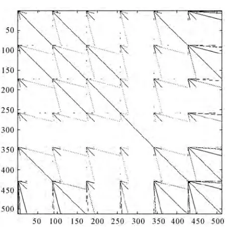
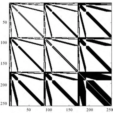
4.1. Wavelet Bases, Decay Estimates and Kernel Sparsification

We present some interesting properties of the wavelet bases introduced in Section 2. In particular we show how the representation in these wavelet bases of certain

classes of linear operators acting on 2



 



0,1

L may be

viewed as a first step for their “compression”, that is as a step to approximate them with sparse matrices. After being compressed these operators can be applied to

arbitrary functions belonging to 2



 



0,1

L in a “fast”

(10)

sparse systems of linear equations and solved at an affordable computational cost. In particular we show how the orthogonality of the wavelet functions to the polynomials up to a given degree (the vanishing moments property) plays a crucial role in producing these sparse approximations.

Let

 

0,1 be the closure of

 

0,1 and  be a

non-negative integer, we denote with C



   

0,1 0,1



the space of the real continuous functions defined on

   

0,1 0,1 -times continuously differentiable on

   

0,1 0,1 . We have:

Theorem 4.1. Let M 1, N2 be two integers,





= 1

J N M, _ _

, 1 , M

N N N M

W _ _



 

0,1



be the set of func-

tions given in (5), and let K x y

 

, ,

 

x y, 

   

0,1 0,1

be a real function such that:

   



0,1 0,1 ,



.

KC  M (39)

Moreover let m, , , j m  , , j, m= 0,1,, m= 0,1,,

= 0,1, ,Nm 1,

   = 0,1,,Nm1,





, = 1, 2, , 1 ,

j j  N M be the following quantities:

 

   

1

, , , , , ₀ _{, , ,} _, 1

0 , , , ,

=

, ,

= 0,1, , = 0,1, , = 0,1, , 1,

= 0,1, , 1, , = 1, 2, , ( 1) ,.

M m j m j _{j m} _N N

M N j m N

m

dx x

dy y K x y

m m N

N j j N M

  _ _                    



     (40)

then there exists a positive constant DM such that we

have:

 





, , , , , 1

, ,

= 0,1, , = 0,1, , = 0,1, , 1,

= 0,1, , 1, , = 1, 2, , ( 1)

M

m j m j M

max m m

m

D N

m m N

N j j N M

        _               (41)

Proof. The proof is analogous to the proof of Pro- position 4.1 in [19]. In fact from (39) it follows that there

exists a positive constant CM such that:

 

,

 

, ,

 

,

   

0,1 0,1 .

M M

M M K x y M K x y C x y

x y

 

   

 

(42)

That is let N, j, j, ,  , m, m be as above

and



x y*, *



be the center of mass of the set







Nm,1 Nm







Nm,



1



Nm



using the

Taylor polynomial of degree M1 of 

 

y =

 

, ,

K x y y

 

0,1 , and base point y=y* when <

m m or the Taylor polynomial of degree M1 of

 

( ) =x K x y( , ), x 0,1 ,

  with base point x=x*, when

> ,

m m Equation (15), the inequality (42) and using the

fact that the functions

, , , , M

N j mN

 and

, , , , M

N j m N

 _{  }

have support in the sets



Nm,



1



Nm



and







Nm, 1 Nm



respectively from the remainder formula of the Taylor polynomial it follows that the esti- mate (41) for m, , , j m  , , j holds. Note that the constant

M

D depends on M, N, N, CM. This concludes the

proof.

For the wavelet basis function having extra vanishing moments, the previous theorem can be improved. That is let  , , , , N

 

M

j m v N x

 and  , , , , N

 

,

M

j m v N y

 _{  } 0,1,m ,

= 0,1, ,

m   = 0,1,,Nm1, = 0,1,,Nm1,





, = 1, 2, , 1 ,

j j  N M be as above, we have:

Theorem 4.2. Let M 1, N2 be two integers,





= 1

J N Mand let *=maxj=1,2,,(N1)M

 

j 0

where the constants _j, j= 1, 2,,



N1



M, are those appearing in (9) and are such that the Equations (6), (7),

(9) (and (3)) are compatible. Let K x y

 

, ,

 

x y, 

   

0,1 0,1 be a real function such that:

   





*

0,1 0,1 , .

KC   M (43)

Moreover let  ,  , N



 

0,1



M N N I M

W   be the set of func-

tions defined in Section 2 and m, , . j m  , , j, m= 0,1,,

= 0,1, ,

m  = 0,1, ,Nm1, = 0,1, ,Nm1,





, = 1, 2, , 1 ,

j j  N M be the following quantities:

 

_{ }



_{   }

1

, , , , , ₀ , , , , 1

, , , , 0

=

, ,

= 0,1, , = 0,1, , = 0,1, , 1,

= 0,1, , 1, , = 1, 2, , ( 1) ,

M N m j m j j m N

M N j m N

m

dx x

dy y K x y

m m N

N j j N M

  _ _                    



     (44)

where  , , , , N

M j m v N

 and  , , , , N

M j m v N

    have, respectively

j

M M and Mj M vanishing moments. Then there

exists a positive constant FM_j,M_j_, such that we have: 

   

 

, , , , , ,

max 1 , 1

= 0,1, , = 0,1, , = 0,1, , 1,

= 0,1, , 1, , = 1, 2, , ( 1) ,

j j

M M m v j m v j

m M m M

m

F N

m m N

N j j N M

                        (45)

Proof. The proof follows the lines of the proof of Theorem 4.1. Going into details, condition (43) implies

that there exists a positive constant *

M

E such that:

 

_,

 

_, * _,

 

_,

   

_0,1 _{0,1 ,}

M M

M

M K x y M K x y E x y