Buffered autoregressive models with conditional heteroscedasticity: An application to exchange rates

(1)

Munich Personal RePEc Archive

Buffered autoregressive models with

conditional heteroscedasticity: An

application to exchange rates

Zhu, Ke and Li, Wai Keung and Yu, Philip L.H.

Chinese Academy of Sciences, University of Hong Kong, University

of Hong Kong

22 February 2014

Online at

https://mpra.ub.uni-muenchen.de/53874/

(2)

Buffered autoregressive models with conditional

heteroscedasticity: An application to exchange rates

BY KEZHU

Institute of Applied Mathematics, Chinese Academy of Sciences, Haidian District,

Zhongguancun, Beijing, China 5

[email protected]

WAIKEUNGLI ANDPHILIPL.H. YU

Department of Statistics and Actuarial Science, University of Hong Kong, Pokfulam Road,

Kowloon, Hong Kong

[email protected] [email protected] 10

ABSTRACT

This paper introduces a new model called the buffered autoregressive model with generalized autoregressive conditional heteroskedasticity (BAR-GARCH). The proposed model, as an exten-sion of the BAR model in Li et al. (2013), can capture the buffering phenomenon of time series in both conditional mean and conditional variance. Thus, it provides us a new way to study the non- 15 linearity of a time series. Compared with the existing AR-GARCH and threshold AR-GARCH models, an application to several exchange rates highlights an interesting interpretation of the buffer zone determined by the fitted BAR-GARCH models.

Some key words: Buffered AR model; Buffered AR-GARCH model; Exchange rate; GARCH model; Nonlinear time

series; Threshold AR model. 20

1. INTRODUCTION

(3)

the references therein for more recent ones. The TAR model with single thresholdrbasically says that the structure of an AR model shifts from one regime to another, if the status of the threshold 25

variableztcrosses above or below the thresholdr. Due to this piecewise linear character, the TAR

model is able to mimic many nonlinear features in time series, such as resonance, limit cycles, time-irreversibility, and many others; see, e.g., Li and Lam (1995), Pesaran and Potter (1997), and Hansen (2011) for an overview. However, in the two-regime situation, there are some cases that the two-way switching of regimes may not happen at the same threshold. A typical example 30

is the hoisting of a typhoon warning signal mentioned in Li et al. (2013). It is observed that a typhoon warning signal is hoisted when the average wind speed up-crosses a certain threshold

rU, but it may only be canceled when the average wind speed down-crosses another threshold rLwhich is smaller thanrU. In view of this, it is reasonable to treat the zone(rL, rU]as a buffer

zone, in which the weather station keeps the warning signal unchanged when the average wind 35

speed (a threshold variable in this case) lies in the buffer zone.

In order to describe such buffering phenomenon in the real world, Li et al. (2013) first in-vestigated a buffered AR (BAR) model. Unlike the TAR model, this BAR model says that the structure of an AR model remains unchanged when the value of zt lies inside the buffer zone

(rL, rU]. Thus, the BAR model provides us a new way to study nonlinearity in time series. As

40

expected, the buffering phenomenon not only exists in meteorology but also in finance and eco-nomics. A nice illustrative example is the study of the quarterly U.S. GNP data set in Li et al. (2013) and Zhu et al. (2013). Their empirical studies showed that the BAR model provides a better fit than TAR model for the GNP series. Based on the fitted BAR model, they discovered an interval of GNP which does not shift in terms of the probabilistic structure unless we have ex-45

perienced a big ‘contraction’ or ‘expansion’ two years before. This finding is clearly of practical interest and can not be detected by the TAR model.

The above-mentioned BAR model focuses on the buffering phenomenon that is present in the

conditional mean. A natural but important extension is to consider the buffering phenomenon in both the conditional mean and variance or in the conditional variance only. It is well known that 50

(4)

model have since been developed to capture the asymmetry and leverage effects in the market volatility. Among them, the threshold GARCH (TGARCH) model proposed by Rabemanjara and 55

Zako¨ıan (1993) and Zako¨ıan (1994) emphasizes that the structures of volatilities are different for positive and negative return series. In their settings, the thresholdr is fixed at zero. Generally, we are interested in cases where the threshold is unknown. Some pioneer works in this context can be found in Li and Li (1996) and Liu et al. (1997), in which the double threshold AR-ARCH and AR-GARCH models were proposed respectively to capture the piecewise linear conditional 60 mean and variance. Motivated by the BAR model, this paper introduces a new model called the buffered AR-GARCH (BAR-GARCH) model. The new model includes the AR-GARCH, dou-ble threshold AR-ARCH, threshold AR-GARCH, or TGARCH model as special cases, and can capture the buffering phenomenon of time series in both conditional mean and variance. To high-light the importance of the BAR-GARCH model, we apply it to several exchange rate series. In 65 most of these cases, the BAR-GARCH model gives a better fit than the AR-GARCH or

TAR-GARCH model. Therefore, the participants in these exchange rate markets should not ignore this buffering phenomenon in the conditional mean/variance or both of them.

This paper is organized as follows. Sections 2 and 3 review the TAR and BAR models, re-spectively. Section 4 proposes our new BAR-GARCH model, with a specified estimation and 70 model-selection procedure. The application of the BAR-GARCH model to several exchange rate series is presented in Section 5. Section 6 concludes with some suggested future work.

2. THE CLASSIC THRESHOLD AUTOREGRESSIVE MODEL

Let{yt}be a stationary time series. Ap-th order threshold autoregressive [TAR(p)] model for

{yt}can be defined as 75

yt= {

φ0+∑p

i=1φiyt−i+εt, ifRt= 1,

ψ0+∑pi=1ψiyt−i+εt, ifRt= 0, (1)

whereRt=I(yt−d≤r) is the regime indicator ofyt, r is the threshold parameter,d(≥1)is

the delay parameter,I(·)is the indicator function, andεtis an uncorrelated error term with zero

mean and variance σ2(>0). Under such a model, there are two separate regimes for yt, and

(5)

each regime. For example, if yt is the daily return on a certain financial asset, model (1) with d= 1andr= 0describes that the structure ofyttoday depends on whether the price rose or fell

on the previous day. This kind of asymmetric phenomenon has been well documented in Li and Lam (1995); see also Tsay (1989, 1998) and Tong (2011) for other empirical studies based on 85

TAR models. Moreover, the TAR model can be treated as a special case of the threshold ARMA (TARMA) model, which also nests TMA model as another special case. A sophisticated study of TMA or TARMA model can be found in Ling and Tong (2005), Li and Li (2008), Li et al. (2011) and Li et al. (2013).

Since the non-linearity ofythappens only when there exists a threshold structure, it is

impor-90

tant for us to detect the existence of a threshold structure. The related works are the Likelihood ratio (LR) test in Chan (1990, 1991), Li and Li (2011) and Zhu and Ling (2012), and the Wald test and Lagrange multiplier (LM) test in Hansen (1996). Once the null hypothesis of no thresh-old structure is rejected, the least squares estimation procedure in Li and Ling (2012) can be used

to estimate model (1). 95

3. THE BUFFERED AUTOREGRESSIVE MODEL

In view of model (1), the regime of yt shifts immediately no matter which directionyt−d

crosses (above or below) the threshold r . However, this may not always be the case. Li et al. (2013) gave several empirical examples to show that the switch in regime may be delayed when

yt−dlies in a buffer zone. To capture this new non-linear feature of time series, they proposed a

100

p-th order buffered autoregressive [BAR(p)] model withRtin (1) satisfying

Rt=  



1 ifyt−d≤rL

0 ifyt−d> rU Rt−1 otherwise

, (2)

whererLandrUare two threshold parameters such thatrL≤rU. This BAR(p) model stipulates

that the regime of yt is unchanged whenyt−d falls into the buffer zone (rL, rU]. WhenrL= rU, the BAR(p) model reduces to the TAR(p) model. As shown in Li et al. (2013), a sufficient

condition for the geometrical ergodicity of the BAR(p) model is

p ∑

i=1

|φi|<1 and p ∑

i=1

|ψi|<1,

(6)

Although both TAR(p) and BAR(p) models have two regimes, the regime indicator in BAR(p) model depends on past observations infinitely far away. This can be illustrated by the fact that 105

Rt(γ) =I(yt−d≤rL) +

∞ ∑

j=1

I(yt−j−d≤rL) j ∏

i=1

I(rL< yt−i+1−d≤rU) a.s.

in BAR(p) models, whereγ = (rL, rU)′. Thus, unlike TAR(p) model, the states of all past

obser-vations{yj;j ≤t−d}have impact on determining the regime of the current observationytin

BAR(p) models. However, given a finite realizations ofyt, the regimes of the first few

observa-tions may not be well identified, since no observaobserva-tions exist fort≤0in practice. To circumvent this problem, it is natural to assume that[rL, rU]is a subset of[a, b], wherea, bare set to some

empirical quantiles of the data sample{yt}nt=1as in Chan (1991) and Andrews (1993). By doing

so, we can always find a smallest integern0(≥p)such thatyn0−dstays outside the region[a, b].

Hence, the regime indicatorRn0(γ)is well identified, and the regime indicators for observations

{yt}nt=n0+1can be iteratively calculated by

Rt(γ) =I(yt−d≤rL) +Rt−1(γ)I(rL< yt−d≤rU).

For the remaining observations{yt}nt=10−1whose regimes are not well identified, we then set their

regime indicators to be zeros. Thus, we should useR˜t(γ)rather thanRt(γ)in practice, where

˜ Rt(γ) =

{

0 fort= 1,· · · , n0−1,

Rt(γ) fort=n0,· · ·, N. (3)

Although the first (n0−1) regime indicators are artificially chosen in (3), efficiency loss is 110 negligible because Zhu et al. (2013) showed thatn0, an integer depending on{yt}nt=1, is bounded

in probability.

Even though the BAR(p) model has two thresholds, it has only two regimes. If we treat the buffer zone as the “middle regime”, the BAR(p) model is similar to the classical three-regime TAR(p) model, but the parameters in its “middle regime” inherit their values from the two outer 115 regimes. Hence, the buffering phenomenon captured by the BAR(p) model can not be handled by the three-regime TAR(p) model. Finally, it is worth noting that the non-linearity ofytin BAR(p)

model exists only when the threshold variablesrLandrU are present. Like the TAR(p) model,

(7)

4. THE BUFFEREDAR-GARCHMODEL

Conditional heteroscedasticity is a key character in most of economic and financial real data. Basically, it says that the conditional variance of the data is changing over time. So far, this phe-nomenon has been well modelled by the ARCH model in Engle (1982) and its huge variants; 125

see, e.g., Bollerslev et al. (1992) and Francq and Zako¨ıan (2010). In many applications, a condi-tional mean model along with an ARCH-type condicondi-tional variance model is necessary to fit the real data (see, e.g., Tsay (2005)). Bollerslev et al. (1992) showed that ignoring the ARCH effect

would lead to inefficient estimates and suboptimal statistical inference in the conditional mean model. In view of this, it is of interest to consider the following buffered AR(p)-GARCH(m, s) 130

(BAR-GARCH) model:

yt= {

φ0+∑pi=1φiyt−i+εt, ifRt= 1, ψ0+∑p

i=1ψiyt−i+εt, ifRt= 0, (4)

whereRtis defined as in (2), and

εt= √

htηt with ht= {

α0+∑mi=1αiε2t−i+ ∑s

i=1βiht−i, ifRt= 1, π0+∑mi=1πiε2_t−i+

∑s

i=1δiht−i, ifRt= 0, (5)

andηtis a sequence of iid random variables with mean zero and variance one. Here, we assume

135

thatα0, π0 >0and otherαi, βi, πi, δi ≥0for the positivity ofht. Particularly, whenrL=rU,

we call models (4)-(5) the threshold AR-GARCH (TAR-GARCH) model which includes the double threshold AR-ARCH model in Li and Li (1996) and Wong and Li (1997, 2000) as a special case. When bothrLandrUare absent, model (4)-(5) becomes the classical AR-GARCH

model. Also, whenp= 0, we have a buffered GARCH model which can be viewed as a natural 140

extension of the threshold GARCH models in Liu, et al. (1997) and Brooks (2001). Thus, when two threshold variables rL and rU in Rt are present and different, the BAR-GARCH model

captures the buffering phenomenon ofytin terms of both conditional mean and variance. Note

that our BAR-GARCH model assumes that both conditional mean and variance models switch regime at the same time. This assumption seems to be the most likely situation in practice, 145

although allowing for different regime-switching rules in the conditional mean and variance models could easily be done.

Next, we consider the estimation for the BAR-GARCH model. Letθ= (θ′

1, θ2′)′ with θ1= (φ′_{, α}′_{, β}′₎′_,_θ

2 = (ψ′, π′, δ′)′,φ= (φ0,· · · , φp)′,ψ= (ψ0,· · · , ψp)′,α= (α0,· · · , αm)′,β=

(β1,· · · , βs)′,π= (π0,· · · , πm)′ andδ= (δ1,· · · , δs)′. Givennobservations ofyt,−2 times

(8)

quasi-log-likelihood of models (4)-(5) (ignoring some constants) can be written as

Ln(θ) = n ∑

t=1

[

loght(θ, γ) + ε2

t(θ, γ) ht(θ, γ) ]

, (6)

whereεt(θ, γ)andht(θ, γ)are iteratively calculated as

εt(θ, γ) = [

yt−φ0− p ∑

i=1 φiyt−i

]

˜ Rt(γ) +

[

yt−ψ0− p ∑

i=1 ψiyt−i

]

(1−R˜t(γ)),

ht(θ, γ) = [

α0+

m ∑

i=1

αiε2t−i(θ, γ) + s ∑

i=1

βiht−i(θ, γ) ]

˜

Rt(γ) 155

+ [ π0+ m ∑ i=1

πiε2t−i(θ, γ) + s ∑

i=1

δiht−i(θ, γ) ]

(1−R˜t(γ))

withR˜t(γ)being defined as in (3) and the initial valuesY0≡ {yi;i≤0}being zeros.

Given(p, m, s, d, γ), the quasi-maximum-likelihood estimatorθˆofθis obtained by minimiz-ingLn(θ) with the Newton-Raphson method. Then, the estimation ofdandγ is employed by

considering 160

min (d,γ)∈Ad×Aγ

Ln(ˆθ),

whereAd={1,· · ·, D} andAγ={(rL, rU);a≤rL≤rU ≤b} for a user-chosen integer D

and two user-chosen real numbersaandb. The spaceAd×Aγcontains all potential candidates

for(d, γ). Furthermore, the estimation ofp, mandsis performed by considering

min (p,m,s)∈Ap×Am×As

AIC(p, m, s), 165

whereAIC(p, m, s) =:Ln(ˆθ) + 2(p+m+s+ 1) is the Akaike information criterion (AIC),

andAp×Am×As =:{0,· · · , P} × {0,· · · , M} × {0,· · ·, S}for some user-chosen integers P, M andS, contains all potential candidates for(p, m, s).

Although the aforementioned estimation procedure ofθand(p, m, s, d, γ)is efficient, it will be very time-consuming. A simple but less efficient way is to first select an efficient TAR- 170 GARCH model (i.e., rL=rU), and then use these estimators for (p, d, m, s) in the

TAR-GARCH model to estimate the parameterθin the BAR-GARCH model. The detailed steps are as follows:

1. Apply the foregoing estimation procedure in model (4)-(5) with rL=rU =r0 to get the

(9)

2. Based on(ˆp,m,ˆ s,ˆ d,ˆrˆ0)from step 1 and each(rL, rU)∈[a,rˆ0]×[ˆr0, b], calculate the

es-timatorθˆ₍rL.rU)forθby minimizingLn(θ)in (6) with the Newton-Raphson method.

3. Obtain the estimators(ˆrL,ˆrU)for(rL, rU)and estimatorθˆ(ˆrL,rˆU)forθvia

(ˆrL,rˆU) := min

(rL,rU)∈[a,rˆ0]×[ˆr0,b]

Ln(ˆθ(rL,rU)).

Note that for the AR-GARCH model, the aforementioned procedure is not needed. It is be-180

cause we do not need to estimate the threshold and delay parameters in this model. Thus, the

AR-GARCH model can be estimated efficiently. Also, it is worth noting that although the esti-mation procedure in steps 1-3 is sub-efficient for the BAR-GARCH model, the TAR-GARCH model estimated from step 1 is nested within the fitted BAR-GARCH model obtained from steps 1-3. Hence, statistical inference about comparing TAR and BAR models in terms of their log-185

likelihood values becomes standard.

5. APPLICATION TO EXCHANGE RATES

In this section, we apply the BAR-GARCH model to fit several exchange rate series. Our main objective is to check whether the BGARCH gives a better fit to the data sets than the AR-GARCH or TAR-AR-GARCH model. If this is the case, practitioners in the exchange rate markets 190

can get more insight from the BAR-GARCH model, which demonstrates that the asymmetric property, caused by a novel buffered mechanism, should not be ignored.

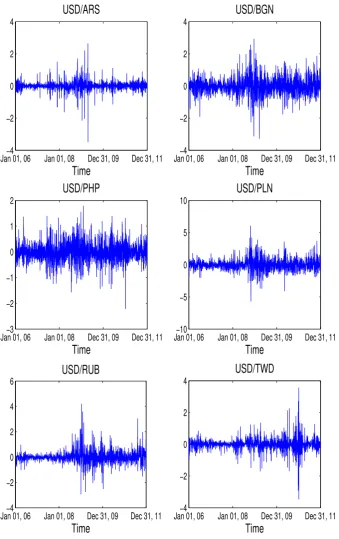
The exchange rate series we studied are the six daily currencies against the U.S. dollar,

the Argentine Peso(USD/ARS), Bulgarian Lev(USD/BGN), Philippine Peso(USD/PHP), Polish Zloty(USD/PLN), Russian Ruble(USD/RUB) and Taiwan Dollar(USD/TWD), over the period 195

from January 1, 2006 to December 31, 2011. They are mostly currencies from developing coun-tries, one from Latin America, two from Asia and three from Eastern Europe. Each series has a total of 2191 observations. The log-return (×100) ytof each series is plotted in Figure 1. A

simple visual inspection of the sample autocorrelation plots ofytandyt2(not reported here)

im-plies that all return series are highly correlated with possible ARCH effect. Thus, it is natural to 200

(10)

most financial applications. The value ofa(orb) is set to be the 10th (or 90th) percentile of the

data. 205

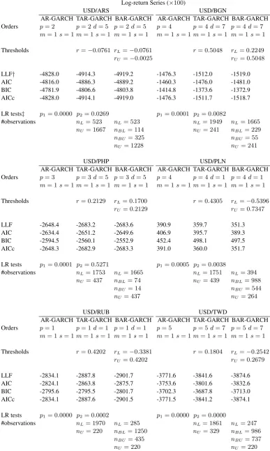
Table 1 reports the estimates for(p, m, s, d, γ)of the best fitted AR-GARCH, TAR-GARCH and BAR-GARCH models for all six exchange rate return series, together with the corresponding values of -2 times the maximized log-likelihood function (LLF), AIC, BIC, and AICc, where LLF is theLn(ˆθ)defined in (6), and

AIC =Ln(ˆθ) + 2k, 210

BIC =Ln(ˆθ) +klog(n),

AICc=Ln(ˆθ) + 2k(k+ 1)/(n−k−1).

Here,kis the number of estimated parameters andnis the sample size. Meanwhile, it is worth mentioning that all best fitted models are adequate by looking at the the ACF and PACF plots (not depicted here) of the residuals and squared residuals. From Table 1, we find that the TAR-GARCH model nests the AR-TAR-GARCH model in all cases. Thus, it is meaningful to use the LR test statistic

LR1n:=LLFAR-GARCH−LLFTAR-GARCH

to test for no threshold structure (i.e., the null is H10: the AR-GARCH model and the alternative

is H11: the TAR-GARCH model). Conventionally, the p-value of LR1nisp1 = 1−Fk1(LR1n)

with k1 =p+m+s+ 4, whereFk(·) is the cdf of a chi-square distribution with degrees of

freedomk. Similarly, we can use the following LR test statistic

LR2n:=LLFTAR-GARCH−LLFBAR-GARCH

to test for no buffer zone (i.e., the null is H20: the TAR-GARCH model and the alternative is

H21: the BAR-GARCH model), and its p-value isp2= 1−F1(LR2n). The values ofp1andp2

for all return series are also given in Table 1, from which we can see that at the 5% level of 215 significance, the TAR-GARCH model is always superior to the AR-GARCH in all cases while the BAR-GARCH model is superior to the TAR-GARCH model except the case of USD/PHP.

To look for further evidence, Table 1 also reports the values of nL,nB andnU, where nB, nLandnU are the number of observations in the buffer zone (i.e.,rL< yt−d≤rU), the lower

(11)

outside the buffer zone (called upper outer regime) (i.e.,yt−d> rU), respectively. Clearly,nBis

zero for all TAR-GARCH models, andnB for a fitted BAR-GARCH model can be decomposed

into nBL andnBU, which are the number of observations in the buffer zone belonging to the

lower and upper regimes, respectively. For the TAR-GARCH models, neithernLnornUis small,

indicating that the threshold effect tends to exist, as also evidenced by significant testing results 225

based on LR1n. For the BAR-GARCH model, most exchange rates except USD/PHP generally

have a large buffer zone, particularly for USD/PLN, USD/RUB and USD/TWD. This implies that the buffer zone exists in most exchange rates except USD/PHP, and this result is consistent with the one based on the likelihood ratio test statistic LR2n. Suppose for instance, the USD/RUB

series is now in the lower regime. According to its fitted BAR-GARCH model, it will move to 230

the upper regime whenever its previous day’s log-return exceeds 0.4202% and then return back to the lower regime only when its previous day’s log-return drops below -0.3381%. However, the TAR-GARCH model will wrongly assign it to the lower regime once its previous day’s log-return

drops below 0.4202%.

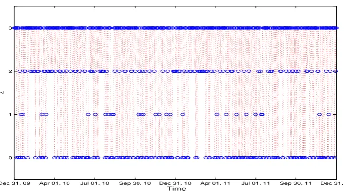
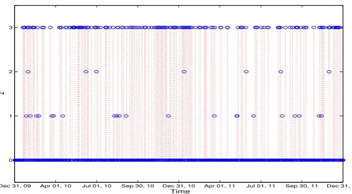
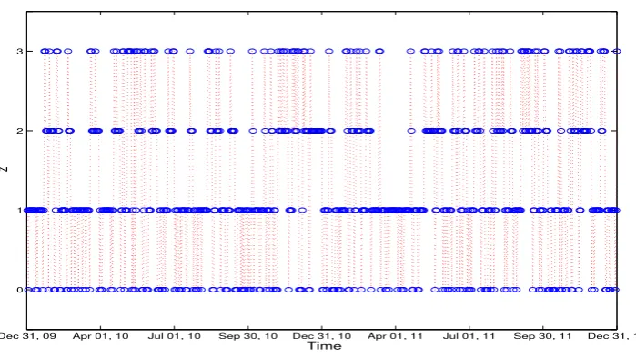
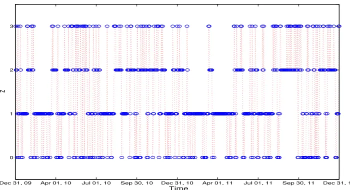
Figures 2-7 plot the time points of each return series belonging to lower outer regime 235

(i.e., yt−d≤rL), lower buffer regime (i.e., rL< yt−d≤rU, Rt= 1), upper buffer regime

(i.e., rL< yt−d≤rU, Rt= 0), and upper outer regime (i.e., yt−d> rU) based on the best fitted

BAR-GARCH model. It can be seen that the USD/PLN, USD/RUB and USD/TWD return series stayed in the buffer zone (lower or upper buffer regimes) most of the time before the financial cri-sis in 2008 but they switched regimes and moved outside the buffer zone more frequently during 240

and after the crisis. This finding reveals that the buffer zone reflects a normal range of exchange rate variation under normal market condition, and the market intervention by the central bank will be invoked only when the exchange rate move outside the buffer zone.

As the hypothesis of no buffer zone is not rejected for USD/PHP, it is natural to see that USD/PHP had very few observations located inside the buffer zone throughout the whole time 245

(12)

[image:12.595.111.499.113.761.2]

Table 1.Model selection results for all six exchange rate return series.

Log-return Series (×100)

USD/ARS USD/BGN

AR-GARCH TAR-GARCH BAR-GARCH AR-GARCH TAR-GARCH BAR-GARCH Orders p= 2 p= 2d= 5 p= 2d= 5 p= 4 p= 4 d= 7 p= 4d= 7

m= 1s= 1m= 1s= 1 m= 1s= 1 m= 1s= 1m= 1s= 1 m= 1 s= 1

Thresholds r=−0.0761 rL=−0.0761 r= 0.5048 rL= 0.2249

rU=−0.0025 rU= 0.5048

LLF† -4828.0 -4914.3 -4919.2 -1476.3 -1512.0 -1519.0 AIC -4816.0 -4886.3 -4889.2 -1460.3 -1476.0 -1481.0 BIC -4781.9 -4806.6 -4803.8 -1414.8 -1373.6 -1372.9 AICc -4828.0 -4914.1 -4919.0 -1476.3 -1511.7 -1518.7

LR tests‡ p1= 0.0000 p2= 0.0269 p1= 0.0001 p2 = 0.0082

#observations nL= 523 nL= 523 nL= 1949 nL= 1665

nU= 1667 nBL= 114 nU= 241 nBL= 229

nBU= 325 nBU = 55

nU= 1228 nU= 241

USD/PHP USD/PLN

m= 1s= 1m= 1s= 1 m= 1s= 1 m= 1s= 1m= 1s= 1 m= 1 s= 1

Thresholds r= 0.2129 rL= 0.1700 r= 0.4305 rL=−0.5396

rU= 0.2129 rU= 0.7347

LLF -2648.4 -2683.2 -2683.6 390.9 359.7 351.3 AIC -2634.4 -2651.2 -2649.6 406.9 395.7 389.3 BIC -2594.5 -2560.1 -2552.9 452.4 498.1 497.5 AICc -2648.3 -2682.9 -2683.3 391.0 360.0 351.7

LR tests p1= 0.0001 p2= 0.5271 p1= 0.0005 p2 = 0.0038

nU= 437 nBL= 74 nU= 439 nBL= 988

nBU= 14 nBU = 544

nU= 437 nU= 264

USD/RUB USD/TWD

m= 1s= 1m= 1s= 1 m= 1s= 1 m= 1s= 1m= 1s= 1 m= 1 s= 1

Thresholds r= 0.4202 rL=−0.3381 r= 0.1804 rL=−0.2542

rU= 0.4202 rU= 0.2679

LLF -2834.1 -2887.8 -2901.7 -3771.6 -3841.6 -3874.6 AIC -2824.1 -2863.8 -2875.7 -3753.6 -3801.6 -3832.6 BIC -2795.6 -2795.5 -2801.7 -3702.3 -3687.8 -3713.0 AICc -2834.1 -2887.6 -2901.5 -3771.5 -3841.2 -3874.1

LR tests p1= 0.0000 p2= 0.0002 p1= 0.0000 p2 = 0.0000

nU= 220 nBL= 1250 nU= 329 nBL= 986

nBU= 435 nBU = 737

nU= 220 nU= 220

†

The smaller value of LLF (AIC, BIC, or AICc), the better fitted model.

‡

(13)

[image:13.595.80.495.106.785.2]

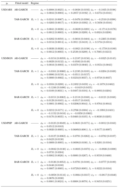
Table 2.Estimated results for the best fitted model of each return series.

yt Fitted model Regime

USD/ARS AR-GARCH ——— φ0= 0.0088 (0.0025)φ1=−0.0838 (0.0193)φ2=−0.1835 (0.0198)

α0= 0.0044 (0.0004)α1= 0.2857 (0.0192)β1 = 0.6754 (0.0161)

TAR-GARCH Rt= 1 φ0= 0.0241 (0.0067)φ1=−0.0476 (0.0398)φ2=−0.2510 (0.0398)

α0= 0.0203 (0.0017)α1= 0.3018 (0.0392)β1 = 0.5656 (0.0344)

Rt= 0 ψ0= 0.0041 (0.0026)ψ1=−0.0639 (0.0201)ψ2=−0.1714 (0.0176)

π0= 0.0012 (0.0003)π1= 0.2698 (0.0209)δ1= 0.6924 (0.0208)

BAR-GARCH Rt= 1 φ0= 0.0202 (0.0058)φ1=−0.0016 (0.0404)φ2=−0.2265 (0.0346)

α0= 0.0154 (0.0014)α1= 0.3911 (0.0418)β1 = 0.5734 (0.0314)

Rt= 0 ψ0= 0.0036 (0.0026)ψ1=−0.0821 (0.0198)ψ2=−0.1759 (0.0180)

π0= 0.0012 (0.0003)π1= 0.2539 (0.0209)δ1= 0.7005 (0.0213)

USD/BGN AR-GARCH ——— φ0=−0.0154 (0.0059)φ1= 0.2187 (0.0156)φ2=−0.0325 (0.0145)

φ3= 0.0029 (0.0132)φ4=−0.0593 (0.0149)

α0= 0.0016 (0.0003)α1= 0.0379 (0.0040)β1 = 0.9554 (0.0043)

TAR-GARCH Rt= 1 φ0=−0.0161 (0.0060)φ1= 0.2195 (0.0185)φ2=−0.0204 (0.0169)

φ3= 0.0086 (0.0159)φ4=−0.0511 (0.0157)

α0= 0.0000 (0.0002)α1= 0.0234(0.0037)β1= 0.9758 (0.0037)

Rt= 0 ψ0= 0.0334 (0.0208)ψ1= 0.2492 (0.0459)ψ2=−0.1679 (0.0462)

ψ3=−0.1246 (0.0486)ψ4=−0.0419 (0.0455)

π0= 0.0189 (0.0031)π1= 0.0487 (0.0104)δ1= 0.8893 (0.0204)

BAR-GARCH Rt= 1 φ0=−0.0151 (0.0062)φ1= 0.2118 (0.0168)φ2=−0.0121 (0.0168)

φ3= 0.0129 (0.0165)φ4=−0.0517 (0.0163)

α0= 0.0001 (0.0002)α1= 0.0206(0.0044)β1= 0.9764 (0.0044)

Rt= 0 ψ0= 0.0212 (0.0171)ψ1= 0.2766 (0.0384)ψ2=−0.1993 (0.0431)

ψ3=−0.1152 (0.0416)ψ4=−0.0350 (0.0363)

π0= 0.0176 (0.0035)π1= 0.0460 (0.0105)δ1= 0.9030 (0.0205)

USD/PHP AR-GARCH ——— φ0=−0.0125 (0.0049)φ1= 0.0631 (0.0171)φ2=−0.0812 (0.0163)

φ3= 0.0512 (0.0163)

α0= 0.0020 (0.0005)α1= 0.0689(0.0081)β1= 0.9177 (0.0097)

TAR-GARCH Rt= 1 φ0=−0.0127 (0.0062)φ1= 0.0791 (0.0262)φ2=−0.0782 (0.0187)

φ3= 0.0423 (0.0130)

α0= 0.0009 (0.0005)α1= 0.0698(0.0100)β1= 0.9201 (0.0104)

Rt= 0 ψ0=−0.0042 (0.0130)ψ1= 0.0035 (0.0373)ψ2=−0.0926 (0.0398)

ψ3= 0.0731 (0.0384)

π0= 0.0082 (0.0026)π1= 0.0000 (0.0267)δ1= 0.9559 (0.0460)

BAR-GARCH Rt= 1 φ0=−0.0126 (0.0052)φ1= 0.0791 (0.0188)φ2=−0.0777 (0.0189)

φ3= 0.0446 (0.0180)

α0= 0.0007 (0.0005)α1= 0.0729(0.0085)β1= 0.9222 (0.0104)

Rt= 0 ψ0=−0.0058 (0.0116)ψ1= 0.0064 (0.0317)ψ2=−0.0817 (0.0340)

ψ3= 0.0676 (0.0330)

(14)

yt Fitted model Regime

USD/PLN AR-GARCH ——— φ0=−0.0280 (0.0091)φ1= 0.2368 (0.0168)φ2=−0.0287 (0.0176)

φ3=−0.0115 (0.0167)φ4=−0.0145 (0.0178)

α0 = 0.0050 (0.0009)α1 = 0.0620 (0.0061)β1= 0.9306 (0.0064)

TAR-GARCH Rt= 1 φ0=−0.0264 (0.0104)φ1= 0.2109 (0.0223)φ2=−0.0055 (0.0178)

φ3=−0.0101 (0.0161)φ4= 0.0022 (0.0164)

α0 = 0.0047 (0.0007)α1 = 0.0339 (0.0076)β1= 0.9289 (0.0071)

Rt= 0 ψ0= 0.0437 (0.0460)ψ1= 0.2198 (0.0461)ψ2=−0.1060 (0.0342)

ψ3=−0.0057 (0.0420)ψ4=−0.0840 (0.0367)

π0= 0.0378 (0.0092)π1= 0.0621 (0.0098)δ1= 0.9379 (0.0223)

BAR-GARCH Rt= 1 φ0=−0.0325 (0.0912)φ1= 0.1949 (0.1087)φ2= 0.0043 (0.1860)

φ3=−0.0560 (0.2370)φ4=−0.0063 (0.5004)

α0 = 0.0065 (0.0891)α1 = 0.0195 (0.1203)β1= 0.9579 (0.4704)

Rt= 0 ψ0=−0.0410 (0.1197)ψ1= 0.2701 (0.5639)ψ2=−0.0718 (0.0278)

ψ3= 0.0600 (0.2954)ψ4=−0.0420 (0.3987)

π0= 0.0000 (0.0989)π1= 0.0768 (0.0118)δ1= 0.9232 (0.9632)

USD/RUB AR-GARCH ——— φ0=−0.0130 (0.0035)φ1= 0.2807 (0.0162)

α0 = 0.0005 (0.0001)α1 = 0.0687 (0.0063)β1= 0.9313 (0.0061)

TAR-GARCH Rt= 1 φ0=−0.0111 (0.0036)φ1= 0.2702 (0.0178)

α0 = 0.0003 (0.0001)α1 = 0.0336(0.0055)β1= 0.9575 (0.0048)

Rt= 0 ψ0=−0.0722 (0.0536)ψ1= 0.3497 (0.0711)

π0= 0.0040 (0.0060)π1= 0.1443 (0.0195)δ1= 0.7254 (0.0361)

BAR-GARCH Rt= 1 φ0=−0.0088 (0.0038)φ1= 0.2766 (0.0202)

α0 = 0.0002 (0.0001)α1 = 0.0265(0.0055)β1= 0.9626 (0.0048)

Rt= 0 ψ0=−0.0123 (0.0114)ψ1= 0.2768 (0.0291)

π0= 0.0053 (0.0009)π1= 0.1088 (0.0118)δ1= 0.8791 (0.0130)

USD/TWD AR-GARCH ——— φ0= 0.0001 (0.0031)φ1=−0.0018 (0.0165)φ2=−0.0801 (0.0174)

φ3=−0.0409 (0.0171)φ4= 0.0450 (0.0155)φ5= 0.0214 (0.0165)

α0 = 0.0007 (0.0001)α1 = 0.0879(0.0070)β1= 0.9121 (0.0062)

TAR-GARCH Rt= 1 φ0= 0.0013 (0.0038)φ1= 0.0105 (0.0253)φ2=−0.0661 (0.0208)

φ3=−0.0239 (0.0186)φ4= 0.0227 (0.0167)φ5= 0.0468 (0.0157)

α0 = 0.0003 (0.0001)α1 = 0.0712(0.0083)β1= 0.9243 (0.0089)

Rt= 0 ψ0= 0.0152 (0.0110)ψ1=−0.0695 (0.0461)ψ2=−0.1064 (0.0452)

ψ3=−0.0184 (0.0482)ψ4= 0.0797 (0.0365)ψ3=−0.1455 (0.0459)

π0= 0.0110 (0.0017)π1= 0.1902 (0.0311)δ1= 0.7587 (0.0407)

BAR-GARCH Rt= 1 φ0=−0.0002 (0.0046)φ1= 0.0132 (0.0265)φ2=−0.0245 (0.0360)

φ3=−0.0328 (0.0243)φ4= 0.0300 (0.0235)φ5= 0.0669 (0.0218)

α0 = 0.0008 (0.0005)α1 = 0.1348(0.0168)β1= 0.8652 (0.0406)

Rt= 0 ψ0= 0.0091 (0.0063)ψ1=−0.0439 (0.0370)ψ2=−0.1015 (0.0282)

ψ3=−0.0192 (0.0243)ψ4= 0.0218 (0.0211)ψ5=−0.0284 (0.0320)

π0= 0.0199 (0.0058)π1= 0.2496 (0.0462)δ1= 0.5678 (0.0934)

†

(15)

Now we consider the parameter estimates of the best fitted models as shown in Table 2. For 250

ease of comparison, we also compute the volatility persistence in each regime derived from these

[image:15.595.77.539.181.253.2]

models (see Table 3).

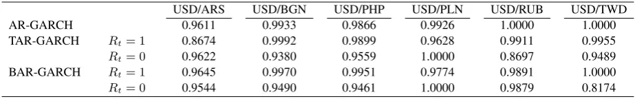
Table 3.Persistence measure in each regime derived from the best fitted models.

USD/ARS USD/BGN USD/PHP USD/PLN USD/RUB USD/TWD

AR-GARCH 0.9611 0.9933 0.9866 0.9926 1.0000 1.0000

TAR-GARCH Rt= 1 0.8674 0.9992 0.9899 0.9628 0.9911 0.9955

Rt= 0 0.9622 0.9380 0.9559 1.0000 0.8697 0.9489 BAR-GARCH Rt= 1 0.9645 0.9970 0.9951 0.9774 0.9891 1.0000

Rt= 0 0.9544 0.9490 0.9461 1.0000 0.9879 0.8174

It can be seen from Table 3 that there was a strong persistence in volatility in all these models,

with a slightly higher persistence in the lower regime in most exchange rates except the case of USD/PLN where it had an explosive volatility in the upper regime. This might be because Poland 255

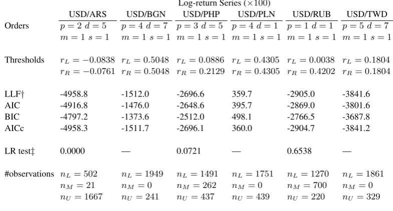
is the only European country to have avoided the recession in the late 2000s (Buckley, 2012). One may argue that as the BAR-GARCH model is nested within the three-regime TAR-GARCH (denoted by 3R-TAR-TAR-GARCH) model, it is therefore interesting to see whether the 3R-TAR-GARCH model can give a better fit to our data sets than the BAR-GARCH model. Ta-ble 4 shows the results of the best fitted 3R-TAR-GARCH model, which is obtained by using the same estimation procedure for the BAR-GARCH model. We also calculate the LR test statistic

LR3n:=LLFBAR-GARCH−LLF3R-TAR-GARCH

to test for the null hypothesis H30: the BAR-GARCH model against the alternative H31: the

3R-TAR-GARCH, and its p-valuep3 = 1−Fk2(LR3n)withk2=p+m+s+ 2.

We can see from Table 4 that for the USD/BGN, USD/PLN and USD/TWD return series, their best fitted 3R-TAR-GARCH models are simply their corresponding two-regime TAR-GARCH 260

models. This indicates that a two-regime model is enough for these three series. For the other three return series, the results of the likelihood ratio test reveal that, at the 5% significance level, the BAR-GARCH model is superior to the 3R-TAR-GARCH model except the USD/ARS return series. However, there are onlynM = 21observations in the middle regime of 3R-TAR-GARCH

model for the USD/ARS return series. In view of this, it is believed that the BAR-GARCH model 265

(16)

[image:16.595.107.500.114.325.2]

Table 4.Model selection results for 3-R-TAR-GARCH model in all six log-return series.

Log-return Series (×100)

USD/ARS USD/BGN USD/PHP USD/PLN USD/RUB USD/TWD Orders p= 2d= 5 p= 4d= 7 p= 3d= 5 p= 4d= 1 p= 1d= 1 p= 5d= 7

m= 1s= 1 m= 1s= 1 m= 1 s= 1 m= 1s= 1 m= 1s= 1 m= 1s= 1

Thresholds rL=−0.0838 rL= 0.5048 rL= 0.0886 rL= 0.4305 rL= 0.0038 rL= 0.1804

rR=−0.0761 rR= 0.5048 rR= 0.2129 rR= 0.4305 rR= 0.4202 rR= 0.1804

LLF† -4958.8 -1512.0 -2696.6 359.7 -2905.0 -3841.6 AIC -4916.8 -1476.0 -2648.6 395.7 -2869.0 -3801.6 BIC -4797.2 -1373.6 -2512.0 498.1 -2766.5 -3687.8 AICc -4958.3 -1511.7 -2696.1 360.0 -2904.7 -3841.2

LR test‡ 0.0000 — 0.0721 — 0.6538 —

#observations nL= 502 nL= 1949 nL= 1491 nL= 1751 nL= 1270 nL= 1861

nM = 21 nM = 0 nM = 262 nM = 0 nM = 700 nM = 0

nU= 1667 nU= 241 nU= 437 nU= 439 nU= 220 nU= 329

†

The smaller value of LLF (AIC, BIC, or AICc), the better fitted model.

‡

The p-values the test statistic LR3n.

6. CONCLUDING REMARKS

This paper proposes a new BAR-GARCH model, which captures the buffering phenomenon of time series in both conditional mean and variance. The empirical study on the six exchange rates series shows that the BAR-GARCH model could provide a better fit than AR-GARCH and 270 TAR-GARCH models in most of cases. It is interesting to find that the buffer zone obtained in these series can be interpreted as a normal region of the exchange rates so that possibly there is no market intervention. All of our findings imply that the property of asymmetry, caused by a novel buffered mechanism from BAR-GARCH model, should not be ignored. Due to the empirical

importance of the BAR-GARCH model, a theoretical exploration on its stationarity, estimation, 275 statistical inference and model-diagnostic, should be considered, and we leave it for a future study.

ACKNOWLEDGEMENT

(17)

REFERENCES

ANDREWS, D.W.K. (1993). Tests for parameter instability and structural change with unknow change point. Econo-metrica61, 821–856.

BOLLERSLEV, T. (1986). Generalized autoregressive conditional heteroskedasticity. Journal of Econometrics31, 285

307–327.

BOLLERSLEV, T., CHOU, R.Y. & KRONER, K.F. (1992). ARCH modelling in finance: A review of the theory and empirical evidence.Journal of Econometrics52, 5–59.

BOLLERSLEV, T. & WOOLDRIDGE, J.M. (1992). Quasi-maximum likelihood estimation of dynamic models with time varying covariance.Econometric Reviews11, 143–172.

290

BROOKS, C. (2001). A double-threshold GARCH model for the French Franc/Deutschmark exchange rate.Journal of Forecasting20, 135–143.

BUCKLEY, N. (2012). Economy: Nation avoided recession but risks persist.Financial Times, June 13, 2012. CHAN, K.S. (1990). Testing for threshold autoregression.Annals of Statistics18, 1886–1894.

CHAN, K.S. (1991). Percentage points of likelihood ratio tests for threshold autoregression. Journal of the Royal

295

Statistical Society Series B53, 691–696.

ENGLE, R.F. (1982). Autoregressive conditional heteroskedasticity with estimates of variance of U.K. inflation.

Econometrica50, 987–1008.

FRANCQ, C. & ZAKO¨IAN, J.M. (2010).GARCH Models: Structure, Statistical Inference and Financial Applications. Chichester, UK: John Wiley.

300

HANSEN, B.E. (1996). Inference when a nuisance parameter is not indentified under the null hypothesis. Economet-rica64, 413–430.

HANSEN, B.E. (2011). Threshold autoregression in economics.Statistics and Its Interface4, 123–127.

LI, G.D., GUAN, B., LI, W.K. & YU, P.L.H. (2013). Buffered threshold autoregressive time series models. Working paper. University of Hong Kong.

305

LI, C.W. & LI, W.K. (1996). On a double-threshold autoregressive heteroscedastic time series model. Jounral of Applied Econometrics11, 253–274.

LI, G.D. & LI, W.K. (2008). Testing for threshold moving average with conditional heteroscedasticity. Statistica Sinica18, 647–665.

LI, G.D. & LI, W.K. (2011). Testing a linear time series models against its threshold extension. Biometrika98, 310

243–250.

LI, D., LI, W.K. & LING, S. (2011). On the least squares estimation of threshold autoregressive and moving-average models.Statistics and Its Interface4, 183–196.

LI, D. & LING, S. (2012). On the least squares estimation of multiple-regime threshold autoregressive models.

Journal of Econometrics167, 240–253. 315

LI, D., LING, S. & LI, W.K. (2013). Asymptotic theory on the least squares estimation of threshold moving-average models.Econometric Theory29, 482–516.

(18)

LING, S. & TONG, H. (2005). Testing a linear MA model against threshold MA models. Annals of Statistics33, 320 2529–2552.

LIU, J., LI, W.K. & LI, C.W. (1997). On a threshold autoregression with conditional heteroscedastic variances.

Journal of Statistical Planning and Inference62, 279–300.

PESARAN, M.H. & POTTER, S.M. (1997). A floor and ceiling model of US output.Journal of Economic Dynamics

and Control21, 661–695. 325

RABEMANJARA, R. & ZAKO¨IAN, J.M. (1993). Threshold ARCH model and asymmetries in volatility. Journal of Applied Econometrics8, 31–49.

TONG, H. (1978). On a threshold model. In Pattern Recognition and Signal Processing (C.H. Chen, ed.) 575-586.

Amsterdam: Sijthoff and Noordhoff.

TONG, H. (1990).Non-linear Time Series. A Dynamical System Approach.Clarendon Press, Oxford. 330 TONG, H. (2011). Threshold models in time series analysis—30 years on (with discussions). Statistics and Its

Interface4, 107–135.

TSAY, R.S. (1989). Testing and modeling threshold autoregressive processes. Journal of American Statistical Asso-ciation84, 231–240.

TSAY, R.S. (1998). Testing and modeling multivariate threshold models.Journal of American Statistical Association 335

93, 1188–1202.

TSAY, R.S. (2005).Analysis of financial time series (2nd ed.). New York: John Wiley & Sons, Incorporated. WONG, C.S. & LI, W.K. (1997). Testing for threshold autoregression with conditional heteroscedasticity.Biometrika

84, 407–418.

WONG, C.S. & LI, W.K. (2000). Testing for double threshold autoregressive conditional heteroscedastic model. 340

Statistica Sinica10, 173–189.

ZAKO¨IAN, J.M. (1994). Threshold heteroskedastic models. Journal of Economic Dynamics and Control18, 931– 955.

ZHU, K. & LING, S. (2012). Likelihood ratio tests for the structural change of an AR(p) model to a threshold AR(p) model.Journal of Time Series Analysis33, 223-232. 345 ZHU, K., YU, P.L.H. & LI, W.K. (2013). Testing for the buffered autoregressive processes. Statistica Sinica.

(19)

Jan 01, 06−4 Jan 01, 08 Dec 31, 09 Dec 31, 11 −2

0 2 4

Time

USD/ARS

Jan 01, 06−4 Jan 01, 08 Dec 31, 09 Dec 31, 11 −2

0 2 4

Time

USD/BGN

Jan 01, 06−3 Jan 01, 08 Dec 31, 09 Dec 31, 11 −2

−1 0 1 2

Time

USD/PHP

Jan 01, 06−10 Jan 01, 08 Dec 31, 09 Dec 31, 11 −5

0 5 10

Time

USD/PLN

Jan 01, 06−4 Jan 01, 08 Dec 31, 09 Dec 31, 11 −2

0 2 4 6

Time

USD/RUB

Jan 01, 06−4 Jan 01, 08 Dec 31, 09 Dec 31, 11 −2

0 2 4

[image:19.595.126.466.121.661.2]

Time

USD/TWD

(20)

Jan 01, 06 Apr 02, 06 Jul 02, 06 Oct 01, 06 Dec 31, 06 Apr 01, 07 Jul 01, 07 Sep 30, 07 Dec 31, 07 0

1 2 3

Time

z

USD/ARS

Jan 01, 08 Apr 01, 08 Jul 01, 08 Sep 30, 08 Dec 30, 08 Mar 31, 09 Jun 30, 09 Sep 29, 09 Dec 30, 09 0

1 2 3

Time

z

Dec 31, 09 Apr 01, 10 Jul 01, 10 Sep 30, 10 Dec 31, 10 Apr 01, 11 Jul 01, 11 Sep 30, 11 Dec 31, 11 0

1 2 3

Time

[image:20.595.136.485.540.733.2]

z

Fig. 2. The time points (represented by circles) in the lower outer regime (i.e., yt−d≤rL), the lower buffering

regime (i.e., rL< yt−d≤rU, Rt= 1), the upper buffering regime (i.e., rL< yt−d≤rU, Rt= 0), and the upper

(21)

1 2 3

Time

z

USD/BGN

1 2 3

Time

z

1 2 3

Time

[image:21.595.118.468.541.735.2]

z

(22)

1 2 3

Time

z

USD/PHP

1 2 3

Time

z

1 2 3

Time

[image:22.595.136.484.541.733.2]

z

(23)

1 2 3

Time

z

USD/PLN

1 2 3

Time

z

1 2 3

Time

[image:23.595.118.468.540.736.2]

z

(24)

1 2 3

Time

z

USD/RUB

1 2 3

Time

z

1 2 3

Time

[image:24.595.135.486.542.732.2]

z

(25)

1 2 3

Time

z

USD/TWD

1 2 3

Time

z

1 2 3

Time

[image:25.595.118.468.542.734.2]

z