The Study on the Phase Structure of the Paul Trap System

(1)

http://www.scirp.org/journal/am ISSN Online: 2152-7393

ISSN Print: 2152-7385

DOI: 10.4236/am.2017.84042 April 28, 2017

The Study on the Phase Structure

of the Paul Trap System

Jaouad Kharbach

1

, Mohamed Benkhali

1

, Mohamed Benmalek

1

, Ahmed Sali

1

,

Abdellah Rezzouk

1

_{, Mohammed Ouazzani-Jamil}

2

1_{Laboratoire de Physique du Solide, Faculté des Sciences Dhar El Mahraz, Université Sidi Mohamed Ben Abdellah,} Fès-Atlas, Morocco

2_{Université Privée de Fès, Laboratoire Systèmes et Environnements Durables, Lot. Quaraouiyine Route Ain Chkef,} Fès, Morocco

Abstract

In this article, the classic dynamic of Paul trap problem is investigated. We give a complete description of the topological structure of Hamiltonian flows on the real phase space. Using the surgery’s theory of Fomenko Liouville tori, all generic bifurcations of the common level sets of the first integrals were de-scribed theoretically. We give also an explicit periodic solution for singular values of the first integrals. Numerical investigations are carried out for all generic bifurcations and we observe order-chaos transition when the critical value of a control parameter is varied.

Keywords

Hamiltonian System, Integrability, Bifurcation, Liouville Tori, Periodic Solutions, Poincaré Section, Chaos

1. Introduction

In recent years, the study of dynamic systems has been undertaken in a wide range of fields, which are located at the crossroads of differential geometry, al-gebraic geometry, number theory, Lie algebra, Intellectual and material means.

A considerable renewed interest appeared for Hamiltonian dynamic systems with two degrees of freedom, one of which is the study of the topological prop-erties of the flow of these systems, their integrability, their chaotic behavior, the study of Periodic solutions and their bifurcation.

A first fundamental task in this field was the search for integrable systems which give rise to non chaotic behavior. For a Hamiltonian system with n de-grees of freedom, the most general definition is that of Liouville. In addition to How to cite this paper: Kharbach, J.,

Benkhali, M., Benmalek, M., Sali1, A., Rez-zouk, A. and Ouazzani-Jamil, M. (2017) The Study on the Phase Structure of the Paul Trap System. Applied Mathematics, 8, 525-536.

https://doi.org/10.4236/am.2017.84042

Received: August 31, 2016 Accepted: April 25, 2017 Published: April 28, 2017

http://creativecommons.org/licenses/by/4.0/

(2)

direct analytical methods, various criteria are developed to determine candidates for integrability, namely the Painlevé criterion, the Ziglin criterion and the Poincaré sections.

Integrability is clearly a central issue in understanding the origins and impli-cations of the behaviour of the dynamical systems. Physically interesting inte-grable systems are rare, and consequently, it stirs up considerable excitement when one is discovered. Moreover, the Painlevé analysis as described in [1] [2] has been contributing -for some time now-a great deal in this direction.

Most integrable problems characterizing the motion of a rigid body around a fixed point were collected in [3], furthermore, the study by Mikhail P. Khar-lamov et al. and A.V. Tsiganov et al., as described in [4] [5] has been contribut-ing for some time already in this direction and others types integrable problems describing the motion of a particle in the Euclidean plane were also collected in the Hietarinta study [6] nevertheless the problems correspond to the trapping of Ions [7] [8], and new integrable problems in this field have been added by many authors.

We examine here an integrable mechanical system which exhibits a great richness of behavior. The proposed system is the system of Paul trap, the Ha-miltonian flows are generated by the HaHa-miltonian:

(

)

1

(

2 2 2

)

1 1

(

2 2 2 2

)

, ,

2 x y z 2

H q p P P P x y z

r

λ

= + + + + + +

λ

₍₁₎

where

λ

is a constant, and 2 2 2

r= x +y +z , is known to be integrable in the following three cases [9]: λ= ±0.5, 1, 2± ± it is also demonstrated that the ion dynamics in a Paul trap can be classified into four dynamical regimes [10]. This classification seems to be rather universal and shows up in the dynamics of pe-riodically perturbed polar molecules, the hydrogen atom in strong magnetic fields [11], and the periodically perturbed hydrogen atom.

The plan of the paper is as follows: In Section 2 we give a detailed description of the real phase space topology of the system (1) in the integrable

λ = ±

1

case,

for doing that, we separate the Hamiltonian system from two canonical trans-formations. This separability implies a description of the topology of the com-mon-level sets of the first integrals (invariant level sets) however, in our study we consider the common-level sets  of the first integrals:

(

)

{

6

}

, , , x, y, z ; ,

x y z P P P H h F f

= ∈ = =

 

 (2)

where H and F are respectively the Hamiltonian and the second invariant of the system.

(3)

527 In the Hamiltonian (1) there is a singularity at

r

=

0

, which necessitates an

infinitesimally small step size for numerical integration of the corresponding equation of motion. So, one has to introduce appropriate coordinate transfor-mation to remove this singularity. For this purpose, you can use two canonical transformations, the first is:

( )

sin

cos , cos

cos

sin , sin

,

x

y

z z

x P P P

y P P P

z z P P

ρ ϕ

ϕ

ρ ϕ ϕ

ρ ϕ

ρ ϕ ϕ

ρ  = = −    ₌ ₌ ₊    = =  (3)

here P P_ρ, _ϕ and P_z are the canonical momenta conjugate to the coordinates

,

ρ ϕ

and z respectively.

Then, Equation (1) Can be rewritten as for

λ = ±

1 (

) (

)

2

2 2 2 2 2 2

2

1 1 1

,

2 z 2 2

P

H P P z r z

r

ϕ

ρ ρ _ρ ρ

= + + + + + = + (4)

Equation (4) is a three degrees of freedom Hamiltonian system in which

ϕ

is a cyclic variable, and so the corresponding canonically conjugate momenta P_ϕ is conserved, or P_ϕ = =m const.

Then, Equation (4) can be rewritten as

(

) (

)

2

2 2 2 2

2

1 1 1

2 z 2 2

m

H P P z

r

ρ ρ _ρ

= + + + + + ₍₅₎

the second canonical transformation is:

( )

sin

cos , cos

cos

sin , sin

r

z r

r P P P

r

z r P P P

r

ρ θ

θ

ρ θ θ

θ θ θ  = = −    = = +  (6)

Then, Equation (5) can be rewritten as

( )

(

)

2

2 2 2

2 ₂ 2

1 1 1 1 1

2 r 2 2 _cos 2

m

H P P r

r

r θ _r _θ

= + + + + (7)

and the Hamilton’s equations of motion of (7) start as

2 3 2 2 d d 1 , d d d d , 0 d d r r r P P r

r P P r

t t r r

P P

P

t r t

θ θ θ θ θ θ  = = = = − +    _{= =} ₌ ₌   

  (8)

which is obtained by making P_ϕ = =m 0.

2. Topological Analysis

In the integrable

λ = ±

1

case, we recall the Hamilton-Jacobi equation

corres-ponding to the system (8) that separates into r,θ coordinates defined by

( )

cos , sin and const

r z r

(4)

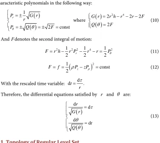
It is easy to check that Pr and Pθ can be expressed in terms of r and

θ

characteristic polynomials in the following way:

( )

1

2 const

r

P G r

r

P_θ Q θ F

 = ±  

 = ± = ± =



where

( )

2 4

2 2 2

2

G r r h r r F

Q θ F

 = − − −

 

=

 (10)

And F denotes the second integral of motion:

2 1 2 2 1 4 1 2

2 r 2 2

F =r h− r P − r − =r Pθ (11)

(

)

2

1

const

2 z

F= =f

ρ

P −zP_ρ = (12)

With the rescaled time variable: dt d . r

τ

=

Therefore, the differential equations satisfied by r and

θ

are:

( )

d d d d r G r t Q τ θ θ  ₌     ₌   (13)

2.1. Topology of Regular Level Set

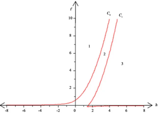
In order to give a complete description of the topology of , we find first the bifurcation diagram B in the

(

h f,

)

-plane, i.e. the set of the critical values of the energy-momentum mapping

(

ρ, ,z P P_ρ, _z

)

→

(

H F,

)

(14)

Definition. The bifurcation diagram of an integrable system is defined to be the region of possible motion depicted on the plane of first integrals

(

h f,

)

[13].

It turns out (like in the Hénon-Heils [14], Gorjatchev-Tchaplygin top [15], Fokker-Planck system [16] [17] and Kolossoff potential [18] [19], the phase to-pology of a special case of Goryachev integrability in rigid body dynamics [20]) that B is exactly the discriminant locus of the polynomial G r

( )

whose coeffi-cients are functions of h and f.

(

)

(

( )

)

{

2

}

, : discriminant 0

B= h f ∈ G r = (15) where

(

_,

)

2_:128 3 _{432 512} 4 ₂₀₄₈ 2 2 ₂₃₀₄ ₂₀₄₈ 3 _0, 1 2 ₀

2 B=_ h f ∈ h − + h f − h f − hf + f = f = P_θ ≥ _

  

[image:4.595.215.541.89.379.2]

The set _ \B consists of three connected components (as it is shown in Figure 1). Thus, in each connected component of the set _\B the level set



 has the same topological type and this latter may be changed only if

(5)

[image:5.595.212.535.71.310.2]

529

Figure 1. Bifurcation diagram B.

As θ is acyclical variable ⇒ ∈θ

[

0, 2π .

]

Theorem. The set _\B consists of three connected and nonintersecting with each other domains. The topological type of  is a disjoint union of two-dimensional two-tori 2T, two-dimensional tori T and the empty set φ.

Proof. Consider the complexified system

(

)

{

4

}

, ; ,

X P H h F f

⊄ = ∈⊄ = =

 (16)

consider also the elliptic curves

( )

{

2

}

1: ω1 G r

Γ = and

{

2

( )

}

2: ω2 Q θ

Γ = (17) and the corresponding Riemann surfaces R1 and R2 of the same genus. We

obtain the explicit solutions of the initial problem (13) by solving the Jacobi in-version problem [21].

Define the natural projection

1 2

:

π

⊄ → Γ ⊗ Γ (18)

(where ⊗ is the symmetric product), and the complex conjugation on ⊄

(

) (

)

: , ,z P P_ρ, _z , ,z P P_ρ, _z

ξ ρ → ρ ₍₁₉₎

Consider also the natural projection

η

on the Riemann surface R=R1⊗R2

given in

( )

r,θ coordinates by η:

( )

r,θ →

( )

r,θ .

It induces an involution on the Jacobi variety and hence on ⊄ by the

nat-ural projection π. By Equations (10) and (13) imply that this involution

η

coincides with the complex conjugation (19) on ⊄. The upshot is that in

or-der to describe  it is enough to study the projection:

( )

1 2

: Jac R

π _⊄ → = Γ ⊗ Γ (20)

Definition. A connected component of the set of fixed points of τ_{on the}

(6)

To determine the ovals of Γ1 and Γ2 it suffices to study the real roots of

the polynomial G r

( )

for different values of h and f as shown in Table 1. Using the Formulae (10), and the condition that

(

_{, ,} _,

)

4

z

z P P_ρ

ρ ∈_ _{we find exactly}

two admissible ovals whose projections on the r–plan and θ −plan are given by ∆1 and ∆2 (see Table 2). The product of the admissible ovals in

1 2

Γ ⊗ Γ _{and the projection}π_of _ such as, 1

(

)

1 2 1 2

π

−

= Γ ⊗ Γ = ∆ × ∆



 ,

gives :

1) is a two-dimensional two-tori 2T in domain 3. 2) is a two-dimensional tori T in domain 2. 3) is the empty set in domain 1.

2.2. Topology of Singular Level Sets

Suppose now that the constants h and f are changed in such a way that

(

h f,

)

passes through the bifurcation diagramB. Then the topological type of  may change and the bifurcation of Liouville tori takes place. In order to describe all ge-neric bifurcations of Liouville tori, we use Fomenko’s theorem of bifurcation for Liouville tori. We can have in our case two types of bifurcation (see Figure 2).

To prove that, it suffices to look at the bifurcations of roots of the polynomial

( )

[image:6.595.230.515.389.567.2]

G r , the correspondence between bifurcation of roots and Liouville tori is shown in Figure 2.

Figure 2. Correspondence between bifurcations of roots of polynomial. G r

( )

and

bi-furcations of invariant Liouville tori.

Table 1. Topological type of  and the real roots of the polynomials G r

( )

for

(

)

2

, \

h f ∈ B.

Domain Real roots of G r( )

1 0

2 r1< <r2 0

[image:6.595.208.538.656.733.2]

(7)

531

[image:7.595.208.540.93.173.2]

∅

Table 2. Admissible ovals and topological type of  for

(

)

2

, \

h f ∈ B.

Domain r–plan∆1 θ–plan∆2 Topological type of 

1 ∅ [0, 2π] ∅

2 [r r1,2] [0, 2π] T

3 [r r1, 2] [ r r3,4] [0, 2π] 2T

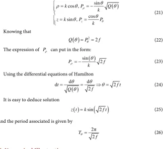
2.3. Periodic Solutions

When the bifurcation of Liouville tori takes place, the level set  becomes completely degenerate. Then we can have exceptional families of periodic solu-tions. It is seen from Table 3 that if

(

h f,

)

is on the smooth curves C0 (see

Figure 1),  contains a isolated circle S which is periodic solution. Consider now a fixed periodic solution belonging to the curve C0. The parameter

θ

takes values in the admissible interval

[

0, 2π

]

and r is equal to the double root of the polynomial G r

( )

, r1= =r2 k (see Table 3).

Then we obtain from (9) and (10) the following parameterization of fixed pe-riodic solution:

( )

sin

cos ,

cos sin , _z

k P Q

k

z k P P

k

ρ

θ

ρ θ θ

θ θ

 = = −

 

 = =



(21)

Knowing that

( )

2

Q

θ

=P_θ = f (22) The expression of Pρ can put in the form:

( )

sin

2

P f

k

ρ

θ

= − (23)

Using the differential equations of Hamilton

( )

d d

d 2

2

t f t

f Q

θ θ _θ

θ

= = ⇒ = ₍₂₄₎

It is easy to deduce solution

( )

sin

(

2

)

z t =k f t (25) and the period associated is given by

2π

2 T

f

θ = (26)

3. Numerical Illustration

Using a surface of the section map, we give numerical illustrations of the topo-logical analysis studied in Section 2.

[image:7.595.210.539.342.642.2]

(8)

(a) (b) (c)

(d) (e) (f)

(g) (h) (i)

(9)

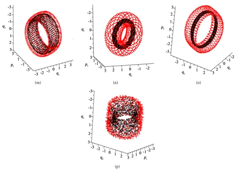
533 (m) (n) (o)

[image:9.595.63.539.64.403.2]

(p)

Figure 3. Surfaces of section map for different values of h, f and λ,

(

q p q p1, 1, 2, 2

) (

= r P, r, ,θ Pθ

)

: (a) Domain 2 (h = 3.016, f =

3.345) _~T; (b) Domain 2 (h = 3.016, f = 4.493) _~T; (c) Domain 2 (h = 3.016, f = 3.345, 4.493, 5.023, 5.156, 5.377)

~T



 ; (d) Domain 2 (h = 3.016, f = 3.345, 4.493, 5.023, 5.156, 5.377) _~T; (e) Domain 2 (h = 3.016,, f = 3.345, 4.493,

5.023, 5.156, 5.377) _~T; (f) Domain 2 (h = 0.718, f = 0.828) _~T; (g) Domain 2 (h = 0.718, f = 0.828) _~T; (h)

Domain 2 (h = 1.997, f = 4.077) _~S; (i) Domain 2 (h = 1.997, f = 4.052) _~S; (j) View 2D of domain 2 (λ = 1.16); (k)

View 3D of domain 2 (λ = 1.16); (l) Domain 2 (λ = 1.35); (m) Domain 3 (h = 4.041, f = 3.017) _~ 2T; (n) Domain 3 (h =

3.128, f = 3.017) _~ 2T; (o) Domain 3 (h = 3.0755, f = 3.017) _ ~TS; (p) View 3D of domain 3 (λ = 1.18).

Table 3. Topological type of  for

(

h f,

)

∈B.

Curve ∆1 ∆2 Topological type of 

0

C {r1=r2} [0, 2π] S

of Liouville tori and the order-chaos transition when one of the system parame-ters is varied. This map is constructed using a clever method introduced by Poincaré and extended by Hénon [22].

(10)

a two-dimensional T.

The fixed points in Figure 3(h) and Figure 3(i) show the sections represent-ing the periodic solution where  is an isolated circle S for h=1.997 and

4.077, 4.052

f = on the curve C0 of B.

The Figure 3(m) show the sections for a value of the first invariant h=4.041 and f =3.017. These values correspond to a point of Domain 3 on the bifurca-tion diagram B where  is a two-dimensional two-tori 2T.

The Figure 3(n) and Figure 3(o) show the sections corresponding to the bi-furcation on the curve C1 of B for h=3.0755, 3.128 and f =3.017 where



 is a TS.

For critical values of a control parameter λ=1.16,1.35,1.18, we observe a fairly random distribution of points which correspond to a dramatic change in the Poincarésections indicating the order-chaos transition, as it is shown respec-tively on the Figure 3(j), Figure 3(k), Figure 3(l), and Figure 3(p).

4. Conclusions

In this study we have treated the classical dynamics of an integrable Hamiltonian system with two degrees of freedom. The system is characterized by a polynomi-al dependent on the invariants of the motion H and F. The different results ob-tained show the capacity of the method used to provide precise information on this Hamiltonian system. We have shown how this system can be converted by canonical transformations to easily exploitable Hamiltonians.

The very important question that we have studied is the topological analysis of the real invariant manifolds of the system. Fomenko’s theory on surgery and bi-furcations of the Liouville tori has been combined with that of the algebraic structure to give a rigorous and detailed description of the topology of the inva-riant manifolds. For noncritical values of H and F, the variety contains torus or is empty.

In the same way we have shown how the periodic orbits can be found for sin-gular values of first integrals, how the period of solutions is determined, and how explicit formulas can be established.

We have also highlighted numerically the topology of the invariant manifolds, the bifurcations of the Liouville tori and the order-chaos transition when the system control parameter varies.

References

[1] Bountis, T.C. (1992) What Can Complex Time Tell Us about Real Time Dynamics. International Journal of Bifurcation and Chaos, 2, 217-228.

https://doi.org/10.1142/S0218127492000239

[2] Ramani, A., Grammaticos, B. and Bountis, T. (1989) The Painleve Property and Singularity Analysis of Integrable and Non-Integrable Systems. Physics Reports, 180, 159-245. https://doi.org/10.1016/0370-1573(89)90024-0

[3] Borisov, A.V. and Mamaev, I.S. (2005) Rigid Body Dynamics. Hamiltonian Meth-ods, Integrability, Chaos. Institute of computer Science, Moscow,576.

(11)

535

Kowalevski-Sokolov Top. Regular and Chaotic Dynamics, 21, 24-65. https://doi.org/10.1134/S1560354716010032

[5] Tsiganov, A.V. (2010) On the Generalized Integrable Chaplygin System. Journal of Mathematical Sciences, 168, 901-911.https://doi.org/10.1007/ s10958-010-0036-5 [6] Hietarinta, J. (1987) Direct Methods for the Search of the Second Invariant. Physics

Reports,147, 87-154.https://doi.org/10.1016/0370-1573(87)90089-5

[7] Yaremko, Y., Przybylska, M. and Maciejewski, A.J. (2015) Dynamics of a Relativistic Charge in the Penning Trap. Chaos: An Interdisciplinary Journal of Nonlinear Sci-ence, 25, 053102-1-16.http://dx.doi.org/10.1063/1. 4919243

[8] Lanchares, V., Pascual, A.I., Palacián, J., Yanguas, P. and Salas, J.P. (2002) Per-turbed Ion Traps: A Generalization of the Three-Dimensional Hénon-Heiles Prob-lem. Chaos: An Interdisciplinary Journal of Nonlinear Science, 12, 87-99.

https://doi.org/10.1063/1.1449957

[9] Baumann, G. and Nonnenmacher, T.F. (1992) Regular and Chaotic Motions in Ion Traps: A Nonlinear Analysis of Trap Equations. Physics Reports, A46, 2682-2692. [10] Blümel, R., Chen, J.M., Diedrich, F., Peik, E., Quint, W., Schleich, W., Shen, Y.R.

and Walther, H. (1988) Phase Transitions of Stored Laser-Cooled Ions. Nature,334, 309-313. https://doi.org/10.1038/334309a0

[11] Wang, D. (2010) Dynamics of a Rydberg Hydrogen Atom in a Generalized van der Waals Potential and a Magnetic Field. Chinese Physics Letters, 27, 2.

[12] Fomenko, A.T. (1988) Integrability and Nonintegrability in Geometric and Me-chanics. Kluwer Academic Publisher,Heidelberg.

https://doi.org/10.1007/978-94-009-3069-8

[13] Bolsinov, A.V., Borisov, A.V. and Mamaev, I.S. (2010) Topology and Stability of In-tegrable Systems. Russian Mathematical Surveys,65, 259-317.

[14] Gavrilov, L. (1989) Bifurcations of the Invariant Manifolds in the Generalised Hé-non-Heils System. Physical,D34, 223-239.

[15] Ouazzani, A.T.H., Kharbach, J., Dekkaki, S. and Ouazzani-Jamil, M. (2000) Bifurca-tions Sets of the Motion of a Heavy Rigid Body around a Fixed Point in Gory-atchev-Tchaplygin Case. IL Nuovo Cimento,115, 1175-1193.

[16] Kharbach, J., Dekkaki, S., Ouazzani, A.T.H. and Ouazzani-Jamil, M. (2001) Topol-ogy and Bifurcations of the Invariant Level Sets of a Fokker-Planck Hamiltonian through Two Coupled Anisotropic Quartic Anharmonic Oscillators. Journal of Physics A: Mathematical and General, 34, 3437-3446.

https://doi.org/10.1088/0305-4470/34/16/312

[17] Kharbach, J., Dekkaki, S., Ouazzani, A.T.H. and Ouazzani-Jamil, M. (2003) Bifurca-tions of the Common Level Sets of Atomic Hydrogen in Van Der Waals Potential. International Journal of Bifurcation and Chaos, 13, 107-114.

https://doi.org/10.1142/S0218127403006364

[18] Gavrilov, L., Ouazzani-Jamil, M. and Caboz, R. (1992) Bifurcations des Tores de Liouville du potentiel de Kolossoff U ρ 1 kcosϕ

ρ

= + − _. _{Comptes Rendus de}

l'Académie des Sciences,315, 289-294.

[19] Gavrilov, L., Ouazzani-Jamil, M. and Caboz, R. (1993) Bifurcation Diagrams and Fomenko's Surgery on Liouville Tori of the Kolossoff Potential U ρ 1 kcosϕ

ρ

= + − _.

Annales scientifiques de l'École normale supérieure, 36, 545-564. https://doi.org/10.24033/asens.1680

(12)

in Rigid Body Dynamics. Sbornik: Mathematics, 205, 1024-1044.

[21] Griffiths, P. and Harris, J. (1994) Principles of Algebraic Geometry. Wiley Inter-science,New York. https://doi.org/10.1002/9781118032527

[22] Hénon, M. (1982) On the Numerical Computation of Poincaré Maps. Physical 5, 412-414. https://doi.org/10.1016/0167-2789(82)90034-3

Submit or recommend next manuscript to SCIRP and we will provide best service for you:

Accepting pre-submission inquiries through Email, Facebook, LinkedIn, Twitter, etc. A wide selection of journals (inclusive of 9 subjects, more than 200 journals)

Providing 24-hour high-quality service User-friendly online submission system Fair and swift peer-review system

Efficient typesetting and proofreading procedure

Display of the result of downloads and visits, as well as the number of cited articles Maximum dissemination of your research work