Munich Personal RePEc Archive
Efficient estimation of heterogeneous
coefficients in panel data models with
common shock
Li, Kunpeng and Lu, Lina
October 2014
Online at
https://mpra.ub.uni-muenchen.de/59312/
Efficient estimation of heterogeneous coefficients in panel
data models with common shocks
∗Kunpeng Li† and Lina Lu‡
First version: December, 2012. This version: October 2014.
Abstract
This paper investigates efficient estimation of heterogeneous coefficients in panel data models with common shocks, which have been a particular focus of recent theo-retical and empirical literature. We propose a new two-step method to estimate the heterogeneous coefficients. In the first step, the maximum likelihood (ML) method is first conducted to estimate the loadings and idiosyncratic variances. The second step estimates the heterogeneous coefficients by using the structural relations implied by the model and replacing the unknown parameters with their ML estimates. We establish the asymptotic theory of our estimator, including consistency, asymptotic representa-tion, and limiting distribution. The two-step estimator is asymptotically efficient in the sense that it has the same limiting distribution as the infeasible generalized least squares (GLS) estimator. Intensive Monte Carlo simulations show that the proposed estimator performs robustly in a variety of data setups.
Key Words: Factor analysis; Block diagonal covariance; Panel data models; Com-mon shocks; Maximum likelihood estimation, heterogeneous coefficients; Inferential theory
∗We thank Jushan Bai, Bernard Salani´e, and participants in seminars at Columbia University, Huazhong University of Science and Technology, Renmin University of China, and University of International Business and Economics for their helpful comments.
†International School of Economics and Management, Capital University of Economics and Business, Beijing, China. Email: [email protected].
1
Introduction
It has been long recognized and well documented in the literature that a small number of factors can explain a large fraction of the comovement of financial, macroeconomic and sectorial variables, for example, Ross (1976), Sargent and Sims (1977), Geweke (1977) and Stock and Watson (1998). Based on this fact, recent econometric literature places particular focus on panel data models with common shocks. These models specify that the dependent variable and explanatory variables both have a factor structure. A typical example can be written as
yit=αi+x′itβi+λ′ift+ǫit,
xit=νi+γi′ft+vit, i= 1,2, . . . , N; t= 1,2, . . . , T.
(1.1)
whereyitdenotes the dependent variable;xitdenotes ak×1 vector of explanatory variables; and ft is an r×1 vector of unknown factors, which represents the unobserved economic shocks. The factor loadings γi and λi capture the heterogeneous responses to the shocks. A salient feature of this paper is that the coefficients of xit are assumed to be individual-dependent. Throughout the paper, we assume that the number of factors is fixed. For the case where the number of factors can increase when the sample size increases, see Li, Li and Shi (2014).
Due to the presence of factor ft, the error term of the y equation (i.e., λ′
ift+ǫit) is correlated with the explanatory variables. The usual estimation methods, such as ordinary least squares method, are not applicable. The instrumental variables (IV) method appears to be an intuitive way to address this issue, but the validity of IV is difficult to justify in practice. A remarkable result from recent studies is that, even without IV, model (1.1) can still be consistently estimated. The related literature includes Pesaran (2006), Bai (2009), Moon and Weidner (2012), Bai and Li (2014), Su, Jin and Zhang (2014) and Song (2013), among others.
Bai (2009) proposes the iterated principal components (PC) method to estimate a model with homogeneous coefficients. His analysis has been reexamined and extended by the perturbation theory in Moon and Weidner (2012). Su, Jin and Zhang (2014) propose a statistic to test the linearity specification of the model. The three studies find that a bias arises from cross-sectional heteroscedasticity. Bai and Li (2014) therefore consider the quasi maximum likelihood method to eliminate this bias from the estimator. All these studies are based on the assumption of homogeneous coefficient. If the underlying coefficients are heterogeneous, misspecification of homogeneity would lead to inconsistent estimation (see the simulation of Kapetanios, Pesaran and Yamagata (2011)).
Song’s methods having their limitations in estimating the heterogeneous coefficients for some particular data setups. The CCE estimator has a reputation for computational sim-plicity and excellent finite sample properties. However, we note that in some cases rank condition alone is not enough for a good approximation. When good approximation breaks down, the CCE estimator would perform poorly. With Song’s method, although his theory is beautiful, the minimizer of the objective function is not easily obtained, especially for the data with heavy cross-sectional heteroscedasticity. As far as we know, there is no good way to address this issue. The limitations of the CCE method and the iterated principal components method are manifested by simulations in Section 6.
Our estimation method is a two-step method. In the first step, we use the maximum likelihood (ML) method to estimate a pure factor model. Next, the heterogeneous coeffi-cients are estimated by using relations implied by the model and replacing the parameters with their ML estimates. The proposed estimation method aims to strike a balance between efficiency and computational economy. We note that in model (1.1) the computational bur-den cannot be ignored due to a great number of βs being estimated, especially when N
is large. This problem is made worse because we can only compute βi (i = 1,2, . . . , N) sequentially, instead of all βi simultaneously by matrix algebra. As a result, the iterated computation method, which requires updatingβi one by one in each iteration, may not be attractive because of the heavy computational burden. Our estimation method overcomes this problem by using the iterated computation method to estimate a pure factor model, delaying the estimation ofβito the second step. Nevertheless, as we will show, the two-step estimators are asymptotically efficient.
The rest of the paper is organized as follows. Section 2 illustrates the idea of our estimation. Section 3 presents some theoretical results of the factor models, in which the covariance matrix of idiosyncratic errors are block-diagonal. These results are very useful for the subsequent analysis. Section 4 presents the asymptotic properties of the proposed estimator. Section 5 extends our method to the case with zero restrictions on the loadings in the y equation. We show that when zero restrictions are present, the loadings contain information forβ. We propose a minimum distance estimator to achieve the efficiency. Section 6 extends the model to nonzero restrictions. Section 7 conducts extensive simulations to investigate the finite sample properties of the proposed estimator and provides some comparisons with the competitors. Section 8 concludes. Throughout the paper, the norm of a vector or matrix is that of Frobenius; that is,kAk= [tr(A′A)]1/2
for matrixA. In addition, we use ˙vt to denotevt−T1 PT
s=1vs for any column vectorvtand
Mwv to denote T1 PTt=1w˙tv˙t′ for any vectorswt and vt.
2
Key idea of the estimation
To illustrate the idea of our estimation, first substitute the second equation of model (1.1) into the first one. Then
"
yit
xit
#
=
"
αi
νi
#
+
"
βi′γi′+λ′i γi′
#
ft+
"
βi′vit+ǫit
vit
#
Letzit= (yit, x′it)′,µi= (αi, νi′)′,uit= (βi′vit+ǫit, vit′ )′ and Λ′ibe the factor loadings matrix beforeft in the above equation. Now we have
zit=µi+ Λ′ift+uit. (2.1) Let Ωi be the covariance matrix of vit and σǫi2 the variance of ǫit. Throughout the paper, we assume that ǫit is independent of vjs for alli, j, t, s. This assumption is crucial to the models with common shocks and is maintained by all the related studies; for example, Bai (2009), Bai and Li (2014), Pesaran (2006), and Moon and Weidner (2012). The covariance ofuit, denoted by Σii, now is
Σii=
"
Σi,11 Σi,12
Σi,21 Σi,22
#
=
"
βi′Ωiβi+σǫi2 βi′Ωi Ωiβi Ωi
#
. (2.2)
This leads to
Σi,22βi = Σi,21. (2.3)
Suppose that we have obtained a consistent estimator of Σii,βi is then estimated by ˆ
βi = ˆΣ−i,221Σˆi,21 (2.4)
We call the above estimator CoVariance estimator, denoted by ˆβiCV since the estimation forβi only involves the covariance ofuit.
The remaining problem is to consistently estimate Σii. A striking feature of the model (2.1) is that the variance matrix of its idiosyncratic errors is block-diagonal. So we need to extend the usual factor analysis to accommodate this feature.
3
Factor models
Leti= 1,2, . . . , N, t= 1,2, . . . , T. Consider the following factor models
zit=µi+ Λ′ift+uit, (3.1)
wherezitis a ¯K×1 vector of observations with ¯K=k+1;uitis a ¯K×1 vector of error terms; Λiis anr×K¯ loading matrix; andftis anr×1 vector of factors. Letzt= (z1′t, z2′t, . . . , z′N t)′,
µ = (µ′1, µ′2, . . . , µ′N)′, Λ = (Λ
1,Λ2, . . . ,ΛN)′ and ut = (u′1t, u′2t, . . . , u′N t)′, then we can rewrite (3.1) as
zt=µ+ Λft+ut. (3.2) Without loss of generality, we assume that ¯f = T−1PT
t=1ft = 0 throughout the paper since the model can be rewritten as zt = µ+ Λ ¯f + Λ(ft−f¯) +ut = µ∗ + Λf∗
t +ut with
µ∗=µ+ Λ ¯f and ft∗=ft−f¯. To analyze (3.2), we make the following assumptions:
Assumption A: The factor ft is a sequence of constants. Let Mff =T−1PTt=1f˙tf˙t′ with ˙ft=ft−T−1PT
t=1ft. We assume thatMff = lim
T→∞Mff is a strictly positive definite matrix.
B.1 uit is independent and identically distributed (i.i.d) over t and uncorrelated over i withE(uit) = 0 and E(ku4itk)≤ ∞for all i= 1,· · · , N andt= 1,· · ·, T. Let Σiibe the variance ofuit and Ψ = diag(Σ11,Σ22, . . . ,ΣN N) be the variance ofut.
B.2 ftis independent of ujsfor all (j, t, s).
Assumption C: There exists a positive constantC sufficiently large such that
C.1 kΛik ≤C for alli= 1,· · · , N.
C.2 C−1 ≤ τmin(Σii) ≤ τmax(Σii) ≤ C for all i = 1,· · · , N, where τmin(·) and τmax(·) denote the smallest and largest eigenvalues of its argument, respectively.
C.3 There exists an r ×r positive matrix Q such that Q = lim N→∞N
−1Λ′Ψ−1Λ, where
Λ = (Λ1,Λ2, . . . ,ΛN)′ and Ψ is the variance of ut= (u′1t, u′2t, . . . , u′N t)′.
Assumption D:The variances Σiifor alliare estimated in a compact set; that is, all
the eigenvalues of ˆΣii are in an interval [C−1, C] for sufficiently large constantC.
Assumptions A-D are usually made in the context of factor analysis; for example, Bai and Li (2012a, 2014). Readers are referred to Bai and Li (2012a) for the related discussions on these assumptions.
3.1 Estimation
The objective function used to estimate (3.2) is
lnL(θ) =− 1
2N ln|Σzz| −
1
2Ntr[MzzΣ
−1
zz ] (3.3)
whereθ= (Λ,Ψ, Mff) and Σzz = ΛMffΛ′+ Ψ;Mzz = T1 PTt=1z˙tz˙t′ is the data matrix where ˙
zt=zt−T1 PTs=1zs. Suppose thatftis random and followsN(0, Mff), the above objective function is the corresponding likelihood function after concentrating out the intercept µ. Although the factorsftare assumed to be fixed constants, we still use the above objective function and call the maximizer ˆθ= (ˆΛ,Ψˆ,Mˆff), defined by
ˆ
θ= argmax θ∈Θ
lnL(θ),
the quasi maximum likelihood estimator, or the MLE, where Θ is the parameter space specified by Assumption D.
It is known in factor analysis that the loadings and factors can only be identified up to a rotation. To see this, let ˆθ = (ˆΛ,Ψˆ,Mˆff) be the maximizer of (3.3), then ˆθ† = (ˆΛ ˆMff1/2,Ψˆ, Ir) is also a qualified maximizer. From this perspective, it is no loss of generality to normalize that
Mff = 1
T
T
X
t=1
ftft′ =Ir.
Under this normalization, Σzz is simplified as Σzz = ΛΛ′+ Ψ.
Maximizing the objective function (3.3) with respect to Λ and Ψ gives the following two first order conditions.
ˆ
Bdiag(Mzz−Σˆzz) = 0 (3.5) where Bdiag(·) is the block-diagonal operator, which puts the element of its argument to zero if the counterpart of Ψ is nonzero, otherwise unspecified. ˆΛ and ˆΨ denote the MLE and ˆΣzz = ˆΛˆΛ′+ ˆΨ.
3.2 Asymptotic properties of the MLE
This section presents the asymptotic results of the MLE for (3.3). Since we only impose
Mff =Ir in (3.2), the loadings and factors still cannot be fully identified. We adopt the treatment of Bai (2003), in which the rotational matrix appears in the asymptotic repre-sentation. This treatment has two advantages in the present context. First, it simplifies our analysis. Second, it clarifies that the estimation and inferential theory of β is invari-ant to the rotational matrix. Alternatively, we can impose some additional restrictions to uniquely fix the rotational matrix; see Bai and Li (2012a) for full identification strategies. The following theorem, which serves as the base for the subsequent analysis, gives the asymptotic representations of the MLE.
Theorem 3.1 Under Assumptions A-D, as N, T → ∞, we have
ˆ
Λi−R′Λi =R′ 1
T
T
X
t=1
ftu′jt+op(T−1/2)
ˆ
Σii−Σii= 1
T
T
X
t=1
(uitu′it−Σii) +op(T−1/2)
where R= Λ′Ψˆ−1Λ(ˆˆ Λ′Ψˆ−1Λ)ˆ −1.
Remark 3.1 Notice that the rotational matrixRonly enters in the asymptotic
representa-tion of ˆΛi. This is consistent with only loadings and factors having rotational indeterminacy and idiosyncratic errors not having such a problem.
Remark 3.2 By the above theorem, we immediately have ˆΛi−R′Λi = Op(T−1/2) and
ˆ
Σii−Σii=Op(T−1/2). These two results continue to hold whenN is fixed since the model falls within the scope of traditional factor analysis. But the asymptotic representations will be more complicated whenN is finite. An implication of this result is that the covariance estimator ˆβiCV is consistent even when N is finite.
4
Asymptotic results for the covariance estimator
Now we use the results in Theorem 3.1 to derive the asymptotic representation of ˆβiCV. Notice ˆβiCV = ( ˆΣi,22)−1Σˆi,21 and βi = (Σi,22)−1Σi,21. Given ˆΣii = Σii+op(1) by Theorem 3.1, the consistency of ˆβi is immediately obtained by the continuous mapping theorem. Furthermore, by Theorem 3.1,
ˆ
Σii−Σii= 1
T
T
X
t=1
Then it follows
ˆ
Σi,21−Σi,21=
1
T
T
X
t=1
[vit(ǫit+vit′ βi)−Ωiβi] +Op(T−1); (4.1)
ˆ
Σi,22−Σi,22=
1
T
T
X
t=1
[vitv′it−Ωi] +Op(T−1). (4.2)
Notice that ˆ
βi−βi= ( ˆΣi,22)−1Σˆi,21−Σ−i,221 Σi,21
= ( ˆΣi,22)−1
h
( ˆΣi,21−Σi,21)−( ˆΣi,22−Σi,22)Σ−i,221 Σi,21
i (4.3)
Substituting (4.1) and (4.2) into (4.3) and noting that ˆΣi,22
p
−
→Ωi and βi = Σ−i,221Σi,21, we
have the following theorem on ˆβiCV.
Theorem 4.1 Under Assumptions A-D, when N, T → ∞, we have
√
T( ˆβiCV −βi) = Ω−i 1
1
√
T
T
X
t=1
vitǫit
+op(1) (4.4)
Remark 4.1 The above asymptotic result implies that our estimator is asymptotically
efficient. To see this, suppose that the factorsftare observed, then the GLS estimator has the asymptotic representation:
√
T( ˆβiGLS −βi) = Ω−i 1
1
√
T
T
X
t=1
vitǫit
+op(1), (4.5)
which is the same as that of Theorem 4.1, implying the asymptotic efficiency of the CV estimator.
Remark 4.2 Although the asymptotic result of ˆβiCV is derived under Assumption B,
we point out that the proposed method works in a very general setup given the results of Bai and Li (2012b), which show that the quasi maximum likelihood method can be used to estimate approximate factor models (Chamberlain and Rothschild, 1983). More specifically, let Σii,t be the variance of uit, where the covariance matrix has an additional superscripttto indicate that it is time-varying. Partition Σii,t as
Σii,t=
"
Σii,t,11 Σii,t,12
Σii,t,21 Σii,t,22
#
.
Under the assumption thatǫit is independent of vit, we have Σii,t,22βi = Σii,t,21 for all t,
which implies that
1
T
T
X
t=1
Σii,t,22
βi= 1
T
T
X
t=1
Σii,t,21.
To consistently estimateβi, it suffices to consistently estimate T1 PTt=1Σii,t. As shown in Bai and Li (2012b), if the underlying covariance is time-varying but misspecified to be time-invariant in the estimation, the resulting estimator of the covariance is a consistent estimator for the average underlying covariance over time, that is, T1 PT
Remark 4.3 For the basic model, the CCE estimator of Pesaran (2006) and the iterated PC estimator of Song (2013) have the same asymptotic representations as in Theorem 4.1 and hence are asymptotically efficient. However, different methods require different conditions for the asymptotic theory. Except for the rank condition, the CCE estimator potentially requiresN be large, otherwise the average error over the cross section cannot be negligible. The PC estimator is derived under the cross-sectional homoscedasticity. If heteroscedasticity is present, a large N is needed to ensure the consistency. For the CV estimator, the consistency can be maintained for a fixed N even in the presence of the cross-sectional heteroscedasticity. So the CV estimator requires the least restrictive condition for the consistency.
Remark 4.4 With slight modification, our method can be used to estimate the
homoge-neous coefficient. Suppose βi ≡ β for all i. Now we have Σi,22β = Σi,21 for all i, which
leads to
XN
i=1
Σi,22
β = N
X
i=1
Σi,21.
So a consistent estimator forβ is
ˆ
β = N
X
i=1
ˆ Σi,22−1
N
X
i=1
ˆ
Σi,21. (4.6)
The asymptotic properties of ˆβ will not be pursued in this paper. In section 6, we conduct a small simulation to examine its finite sample performance.
Corollary 4.1 Under the assumptions of Theorem 4.1, we have
√
T( ˆβiCV −βi)→−d N 0, σ2ǫiΩ−i 1
,
where σ2ǫi is the variance of ǫit and Ωi is the variance of vit. The variance σǫi2Ω−i 1 can be
consistently estimated by σˆǫi2Σˆ−i,221 , where σˆǫi2 = ˆΣi,11−βˆCVi ′Σˆi,22βˆiCV.
5
Models with zero restrictions
In this section, we consider the following restricted model:
yit=αi+x′itβi+ψi′gt+ǫit
xit=νi+γig′gt+γih′ht+vit
(5.1)
where the dimensions ofgt and ht are r1×1 and r2×1, respectively. A salient feature of
model (5.1) is that the explanatory variables include more factors than the error of the y
variables. In model (5.1), gt denotes the endogenous shocks that directly affect y and x, and ht denotes the exogenous shocks that affect firstx theny①.
The y equation of (5.1) can be written as
yit =αi+x′itβi+ψi′gt+φ′iht+ǫit
withφi= 0 for all i. Letft= (gt′, h′t)′,λi = (ψ′i, φ′i)′ and γi = (γig′, γih′)′, we have the same representation as (1.1). From this perspective, model (5.1) can be viewed as a restricted version of model (1.1). This implies that the two-step method proposed in Section 4 is applicable to (5.1). However, this estimation method is not efficient. Consider the ideal case thatgt is observable. To eliminate the endogenous ingredient ψi′gt, we post-multiply
MG=I−G(G′G)−1G′ on both sides of theyequation. The remaining part ofxit includes
vit and γih′(ht−H′G(G′G)−1gt), which both provide the information for β. However, as shown in Theorem 4.1, only the variations ofvit are used to signalβi in ˆβiCV. Therefore, partial information is discarded and the two-step method in Section 4 is inefficient.
The preceding discussion provides some insights on the improvement of efficiency. To efficiently estimate model (5.1), we need to use information contained in the common components ofxit. Rewrite model (5.1) as
"
yit
xit
#
=
"
αi
νi
#
+
"
βi′γig′+ψi′ βi′γih′ γig′ γih′
# "
gt
ht
#
+
"
βi′vit+ǫit
vit
#
(5.2)
We use Λ′
i to denote the loadings matrix before ft= (g′t, h′t)′. The symbols µi,zit and uit are defined the same as in the previous section. We then have the same equation as (2.1). Further partition the loadings matrix Λi into four blocks,
Λi=
"
Λi,11 Λi,12
Λi,21 Λi,22
#
=
"
ψi+γigβi γig
γihβi γih
#
. (5.3)
So we have Λi,22βi = Λi,21. This result together with (2.3) leads to
"
Λi,22
Σi,22
#
βi=
"
Λi,21
Σi,21
#
(5.4)
Given the above structural relationship, a routine to estimateβiis replacing Λi,22,Λi,21,Σi,22
and Σi,21 with their MLE and minimizing the distance on the both sides of the equation
with some weighting matrix. While this method is intuitive, it is not correct since ˆΛi,22
and ˆΛi,21 are not consistent estimators of Λi,22 and Λi,21, as shown in Theorem 3.1. Let
Λ∗
i =R′Λi represent the underlying parameters that the MLE corresponds to, where R is the rotation matrix defined in Theorem 3.1. Then
Λ∗′i =
"
Λ∗′
i,11 Λ∗′i,21
Λ∗′
i,12 Λ∗′i,22
#
= Λ′iR=
"
Λ′
i,11 Λ′i,21
Λ′
i,12 Λ′i,22
# "
R11 R12
R21 R22
#
=
"
βi′γig′+ψ′i βi′γih′ γig′ γh′
i
# "
R11 R12
R21 R22
#
①
Another way to see this point is as follows. Notice that thexequation can always be written as
xit=νi+ (γig′+γ h′
i H
′
G(G′G)−1)gt+γih′(ht−H
′
G(G′G)−1gt) +vit=νi+γi∗g′gt+γih′h
∗
t +vit.
In the last equation,gtis uncorrelated withh∗t. Given this expression, it is no loss of generality to assume
thatht is uncorrelated withgt. Now we see thatgt causes the endogeneity problem butht does not. So
implying
Λ∗i,21= (R′12γig+R22′ γih)βi+R′12ψi (5.5) Λi,∗22=R12′ γig+R′22γih (5.6) From (5.5) and (5.6), we see that unless ψi = 0, Λ∗i,22βi = Λ∗i,21 does not hold. But
when ψi = 0, we see from (5.1) that the model is free of the endogeneity problem and the ordinary least squares method is applicable. The preceding analysis indicates that the existence of the rotational indeterminacy for loadings impedes the use of the underlying relation Λi,22βi= Λi,21 in the estimation ofβi.
Although this result is a little disappointing, we now show that with some transforma-tion, Λi,22βi= Λi,21 can still be used to estimateβi. First by Λ∗′i = Λ′iR,
Λ∗i,11= (R′11γig+R21′ γih)βi+R′11ψi (5.7) Λi,∗12=R11′ γig+R′21γih (5.8) By the expressions (5.5)-(5.8), we have the following equation:
(Λ∗i,21−Λ∗i,22βi) =R′12R′−111(Λ∗i,11−Λ∗i,12βi) =V(Λi,∗11−Λ∗i,12βi) (5.9) whereV =R′
12R′−111, an r2×r1 rotational matrix. The preceding equation can be written
as
(Λ∗
i,22−VΛ∗i,12)βi= Λ∗i,21−VΛ∗i,11 (5.10)
Given the above result, together with (2.3), we have
"
Λ∗
i,22−VΛ∗i,12
Σi,22
#
βi=
"
Λ∗
i,21−VΛ∗i,11
Σi,21
#
(5.11)
IfV is known, then we can replace Λ∗
i,11,Λ∗i,12,Λ∗i,21,Λ∗i,22with the corresponding estimates,
and βi is efficiently estimated. AlthoughV is unknown, it can be consistently estimated by (5.9) sinceβi can be consistently (albeit not efficiently) estimated by ˆβiCV = ˆΣi,−221 Σˆi,21.
Given the above analysis, we propose the following estimation procedure:
1. Use the maximum likelihood method to obtain the estimatesΣˆii,Λˆi,fˆt for all iandt.
2. Calculate βˆiCV = ˆΣ−i,221Σˆi,21 and
ˆ
V =h N
X
i=1
(ˆΛi,21−Λˆi,22βˆiCV)(ˆΛi,11−Λˆi,12βˆiCV)′
ihXN
i=1
(ˆΛi,11−Λˆi,12βˆiCV)(ˆΛi,11−Λˆi,12βˆCVi )′
i−1
.
3. Calculate βˆi = ( ˆ∆′iWi−1∆ˆi)−1∆ˆ′iWi−1δˆi, where Wi is a predetermined weighting
ma-trix that is specified below, and
ˆ ∆i =
"ˆ
Λi,22−VˆΛˆi,12
ˆ Σi,22
#
, δˆi=
"ˆ
Λi,21−VˆΛˆi,11
ˆ Σi,21
#
(5.12)
where we call the resulting estimator the Loading-coVariance estimators, denoted by
ˆ
Remark 5.1 We can iterate the second and third steps by using the updated estimator of βi to calculate ˆV. We call the estimator resulting from this iterating procedure the
Iterated-LV estimator, denoted by ˆβiILV. The iterated estimator has the same asymptotic representation as the LV estimator, but better finite sample performance; see the simulation results in Section 6.
5.1 The optimal weighting matrix
To carry out the estimation procedure, we need to specify the weighting matrixWi. It can be shown that the theoretically optimal weighting matrix is
Wiopt=
"
R′22·1Mhh−1·gR22·1 0r2×k 0k×r2 Σi,22
#
,
whereR22·1 =R22−R21R−111R12andMhh·g =Mhh−MhgMgg−1Mgh. This weighting matrix can be consistently estimated by
ˆ
Wi =
h
1
T
PT
t=1hˆtˆh′t
− T1
PT
t=1ˆhtηˆt′
1
T
PT
t=1ηˆtηˆt′
−1 1
T
PT
t=1ηˆtˆh′t
i−1
0r2×k 0k×r2 Σˆi,22
(5.13)
with ˆηt= ˆgt+ ˆV′ˆht, where ˆgtand ˆhtare given by
"
ˆ
gt ˆ
ht
#
= N
X
i=1
ˆ
ΛiΣˆ−ii1Λˆ′i
−1XN
i=1
ˆ
ΛiΣˆ−ii1zit
.
5.2 The asymptotic result
The following theorem gives the asymptotic representation of the LV estimator with some remarks following.
Theorem 5.1 Under Assumptions A-D, when N, T → ∞, we have
√
T( ˆβiLV −βi) = γih′(Mhh−MhgMgg−1Mgh)γih+ Ωi−1
×√1
T
T
X
t=1
h
γih′ h˙t−MhgMgg−1g˙t+vit
i
ǫit+op(1)
Given Theorem 5.1, we have the following corollary:
Corollary 5.1 Under the assumptions of Theorem 5.1, we have
√
T( ˆβiLV −βi)→−d N 0, σǫi2(γih′Mhh·gγih+ Ωi)−1.
where Mhh·g = plim T→∞
(Mhh−MhgM−1
gg Mgh). The above asymptotic result can be presented
alternatively as
√
T( ˆβiLV −βi)−→d N 0, σ2ǫi
plim T→∞
1
TX
′
iMGXi
−1
.
Remark 5.2 Consider the “y” equation, which can be written as
Yi=αi1T +Xiβi+Gψi+Ei (5.14) whereYi = (yi1, yi2, . . . , yiT)′,Xi= (xi1, xi2, . . . , xiT)′, and Ei is defined similarly as Yi. If the factorsgt are observable, the infeasible GLS estimator forβi is
ˆ
βiGLS = (Xi′MGXi)−1(Xi′MGYi). By (5.14), we have
ˆ
βiGLS −βi = (Xi′MGXi)−1(Xi′MGEi).
Notice var(Ei) =σǫi2IT. Thus the limiting distribution of ˆβiGLS−βi conditional onXi is
√
T( ˆβiGLS−βi)−→d N 0, σ2ǫi
plim T→∞
1
TX
′
iMGXi
−1
.
the same as that of Corollary (5.1). This means that the LV estimator ˆβiLV is asymptotically efficient.
Remark 5.3 Consider the following model, in which zero restrictions exist in both the x
equation and the y equation:
yit=αi+x′itβi+ψi′gt+ǫit
xit=νi+γih′ht+vit
(5.15)
where gt and ht are assumed to be correlated. Model (5.15) is a special case of (5.1) in view that γig is restricted to zero. So the loading-covariance two-step method can be directly applied to (5.15). We note that the LV estimator is efficient even in the presence of additional zero restrictionsγig = 0. To see this point, notice that Λi in model (5.15) is
Λi =
"
Λi,11 Λi,12
Λi,21 Λi,22
#
=
"
ψi 0
γihβi γih
#
.
The coefficient βi can only be estimated by the relations of Λi,21 and Λi,22, which is the
same as Model (5.1). By the same arguments, we conclude that the model
yit=αi+x′itβi+ψ′igt+φ′iht+ǫit,
xit=νi+γih′ht+vit. is efficiently estimated by the CV method.
Remark 5.4 If the underlying coefficients are identical, we can also use the information
contained in the loadings to improve the efficiency. Let
ˆ
gi(V, β) =
"
ˆ
Λi,22−VΛˆi,12
ˆ Σi,22
#
β−
"
ˆ
Λi,21−VΛˆi,11
ˆ Σi,21
#
.
Given equation (5.11) (notice that nowβi≡β for all i) we can consistently estimate β by
( ˆβLV,Vˆ) = argmin β,V
N
X
i=1
ˆ
where ˆWi is defined in (5.13). Notice that if Λ is identified, we can estimate β by (5.4), replacing the unknown parameters with their estimates. So the additional estimation of
V can be regarded as the cost we pay for the rotational indeterminacy. The finite sample properties of the above LV estimator will be investigated in Section 7.
6
Discussions on models with time-invariant regressors
In some applications, it is of interest to include some time-invariant variables, such as gender, race, education, and so forth. In this section, we address this concern. Consider the following model with time-invariant variables:
yit=αi+x′itβi+ψi′gt+φ′iht+ǫit xit=νi+γig′gt+γih′ht+vit
(6.1)
whereφi’s are observable and represent the time-invariant regressors. Model (6.1) specifies that the coefficients ofφi are time-varying. We believe that this is a sensible way to make the model flexible enough. Now we show that our estimation idea can be used to estimate (6.1). As in the previous section, rewrite model (6.1) as
"
yit
xit
#
=
"
αi
νi
#
+
"
β′
iγgi′+ψ′i βi′γih′+φ′i
γig′ γih′
# "
gt
ht
#
+
"
β′
ivit+ǫit
vit
#
(6.2)
Let Λ′
ibe the loadings matrix beforeft= (gt′, h′t)′ and partition it into four blocks, we have Λi =
"
Λi,11 Λi,12
Λi,21 Λi,22
#
=
"
ψi+γgiβi γig
φi+γihβi γih
#
(6.3)
Let Λ∗
i = R′Λi be the underlying parameters that the estimators correspond to. So we have
Λ∗′i =
"
Λ∗′
i,11 Λ∗′i,21
Λ∗′
i,12 Λ∗′i,22
#
= Λ′iR=
"
Λ′
i,11 Λ′i,21
Λ′
i,12 Λ′i,22
# "
R11 R12
R21 R22
#
This leads to
Λ∗i,11 = (R′
11γig+R′21γih)βi+R′11ψi+R21′ φi, Λ∗i,12 =R11′ γig+R21′ γih (6.4) Λ∗i,21 = (R′
12γig+R′22γih)βi+R′12ψi+R22′ φi, Λ∗i,22 =R12′ γig+R22′ γih (6.5) From (6.4)−(6.5), we have
R12′ R′−111(Λi,∗11−Λ∗i,12βi) +R′22·1φi= (Λ∗i,21−Λ∗i,22βi) (6.6) whereR22·1=R22−R21R11−1R12. Given (6.6) together with Σi,22βi = Σi,21, we have
"
Λ∗
i,22−VΛ∗i,12
Σi,22
#
βi =
"
Λ∗
i,21−VΛ∗i,11−R′22·1φi Σi,21
#
(6.7)
whereV =R′
12R′−111. IfV and R22·1 are known, we can use (6.7) to efficiently estimateβi. Similarly as in the previous section, we can use ˆβCVi to get a preliminary estimators for V
1. Use the maximum likelihood method to obtain the estimates Σˆii,Λˆi and fˆt for all i
andt.
2. Calculate βˆiCV = ˆΣ−i,221Σˆi,21 and Vˆ and Rˆ22·1 by
[ ˆV ,Rˆ′22·1] =h N
X
i=1
(ˆΛi,21−Λˆi,22βˆCVi )Ξi
ihXN
i=1
ΞiΞ′i
i−1
where Ξi= [(ˆΛi,11−Λˆi,12βˆiCV)′, φ′i]′.
3. Calculate βˆiLV = ( ˆ∆′
iWˆi−1∆ˆi)−1∆ˆ′iWˆi−1γˆi, where ˆ
∆i =
"ˆ
Λi,22−VˆΛˆi,12
ˆ Σi,22
#
, γˆi =
"ˆ
Λi,21−VˆΛˆi,11−Rˆ22′ ·1φi ˆ
Σi,21
#
andWˆi is the predetermined weighting matrix, which is the same as (5.13).
Similarly we can iterate Steps 2 and 3 by replacing ˆβiCV with the updated LV estimator. This leads to the iterated LV estimator. Under the same conditions of Theorem (5.1), we can show
√
T( ˆβiLV −βi) = γih′(Mhh−MhgMgg−1Mgh)γih+ Ωi−1
×√1
T
T
X
t=1
h
γih′ h˙t−MhgMgg−1g˙t+vit
i
ǫit+op(1)
The above asymptotic result can be interpreted in a similar way as in Remark 5.2. So the LV estimator is asymptotically efficient.
7
Finite sample properties
In this section, we run Monte Carlo simulations to investigate the finite sample proper-ties of the proposed estimators. The model considered in the simulation consists of one explanatory variable (K= 1) and two factors (r= 2), which can be presented as
yit=αi+xitβi+ψigt+φiht+ǫit,
xit=νi+γiggt+γihht+vit,
(7.1)
wheregt and ht are both scalars. We consider the following different specifications on the models (M), loadings (L), errors (E) and coefficients(C):
M1: ψi and φi are random variables for alli;
M2: φi is zero for all iand ψi is a random variable.
L1: ψi and φi (if not zero) are generated according to ψi = 2 +N(0,1) and φi = 1 +N(0,1); similarlyγig and γih are generated by γig = 1 +N(0,1) and γih = 2 +N(0,1).
L2: ψi and φi (if not zero) are generated from N(0,1); γig and γih are generated according toγig =ψi+N(0,1) and γhi =φi+N(0,1).
Υi = diag(1,(Mi′Mi)−1/2Mi) with Mi being a K×K standard normal random matrix. Let ςit = (ǫit, vit)′ and ςt = (ς1′t, ς2′t, . . . , ςN t′ )′. Then ςt is generated according to ςt =
p
diag(Ξ)Υεt, where εtis an N(K+ 1)×1 vector with all its elements generated i.i.d from
N(0,1).
E2: Let
Li =
"
ψi φi
γig γih
#
, i= 1,2, . . . , N
and L= (L′1, L′2, . . . , LN′ )′ an N(K+ 1)×2 matrix. ς
t is generated as inE1except that
Ξi= 0.1 +
ηi
1−ηi
ι′iιi, i= 1,2,· · ·, N(K+ 1)
whereι′
i is the ith row ofL, andηi is drawn independently from U[u,1−u] with u= 0.1.
C1: βi = 1 +N(0,0.04) for alli.
C2: βi = 1 for alli.
Remark 7.1 Two specifications in M denotes the two models considered in the paper.
M1 corresponds to the basic model, and M2 corresponds to the model with zero restric-tions. We consider two different sets of loadings, L1 and L2. Both specifications give rise to the endogeneity problem in the y equation, but as will be seen below, the CCE esti-mator performs quite differently in the two setups. We also consider the cross-sectional homoscedasticity and heteroscedasticity in the simulation, which correspond to E1 and E2, respectively. When generating heteroscedasticity, we add 0.1 to the expression, avoiding the variance being too close to zero. Our approach to generating the idiosyncratic errors is similar to Doz, Giannone and Reichlin (2012) and Bai and Li (2014). We also consider two specifications for the coefficients. While we mainly focus on the performance of the esti-mation of heterogeneous coefficients, we also use simulations to examine the finite sample properties of the two estimators proposed in Remarks 4.4 and 5.4.
The other parameters includinggt, ht, αi, νiare all generated independently fromN(0,1). To evaluate the performance of estimators, we use the average of the root mean square error (RMSE) to measure the goodness-of-fit, which is calculated by
v u u t 1
NS
S X
s=1
N
X
i=1
( ˆβi(s)−βi)2,
where ˆβi(s) is the estimator of theith unit in the sth experiment, andβi is the underlying true value. S is the number of repetitions, which is set to 1000 in the simulation.
7.1 Determining the number of factors
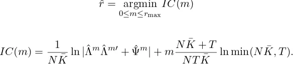
consistent with the theory established in Section 3, we instead consider the following MLE-based information criterion in the simulation
ˆ
r= argmin
0≤m≤rmax
IC(m) (7.2)
where
IC(m) = 1
NK¯ ln|
ˆ
ΛmΛˆm′+ ˆΨm|+mNK¯ +T
N TK¯ ln min(N
¯
K, T).
where ˆΛm and ˆΨm are the respective estimators of Λ and Ψ when the number of factors is set to m and ¯K =K + 1. For the model with zero restrictions, we need to determine the factor numbers in they equation and the x equation, respectively. Following Bai and Li (2014), we consider a two-step method to determine them. First, we use (7.2) to obtain the total numberr=r1+r2, denoted by ˆr, and the associated CV estimator ˆβirˆ; we then use (7.2) again to determine the factor number of the residual matrix R = (Rit) with Rit= ˙yit−x˙′
itβˆiˆr, which we use ˆr1 to denote. Then ˆr2 = ˆr−ˆr1. In the simulation, we set
rmax= 3.
In practice, the basic model and the model with zero restrictions cannot be differenti-ated. We therefore suggest estimating the two models in a unified way. More specifically, for a given data set, we calculater andr1. If ˆr= ˆr1, we turn to the basic model; if ˆr >rˆ1,
[image:17.612.160.452.116.180.2]we turn to the model with zero restrictions.
Table 1 reports the percentages that the number of factors is correctly estimated by (7.2) based on 1000 repetitions. From the table, we see that the number of factors can be correctly estimated with very high probability. This result is robust to all combinations of listed specifications on loadings, errors and models.
Table 1: The percentage of correctly estimating the number of factors
M1 M2
T 50 100 150 200 50 100 150 200
L1+E1 L1+E1
N
50 99.9 100.0 100.0 100.0 100.0 100.0 100.0 100.0 100 100.0 100.0 100.0 100.0 100.0 100.0 100.0 100.0 150 100.0 100.0 100.0 100.0 100.0 100.0 100.0 100.0
L1+E2 L1+E2
N
50 100.0 100.0 100.0 100.0 100.0 100.0 100.0 100.0 100 100.0 100.0 100.0 100.0 100.0 100.0 100.0 100.0 150 100.0 100.0 100.0 100.0 100.0 100.0 100.0 100.0
L2+E1 L2+E1
N
50 99.8 100.0 100.0 100.0 99.9 100.0 100.0 100.0 100 100.0 100.0 100.0 100.0 100.0 100.0 100.0 100.0 150 100.0 100.0 100.0 100.0 100.0 100.0 100.0 100.0
L2+E2 L2+E2
N
[image:17.612.136.478.455.721.2]7.2 Finite sample properties of several estimators
In this section, we examine the performance of the CV and LV estimators. For the purpose of comparison, we also calculate Pesaran’s CCE estimator, Song’s PC estimator, and the infeasible GLS estimator. The infeasible GLS estimator, which is calculated by assuming that the factors are observed, serves as the benchmark for comparison. Since the previous subsection has confirmed that the number of factors can be correctly estimated with high probability, we assume that the number of factors is known in this subsection.
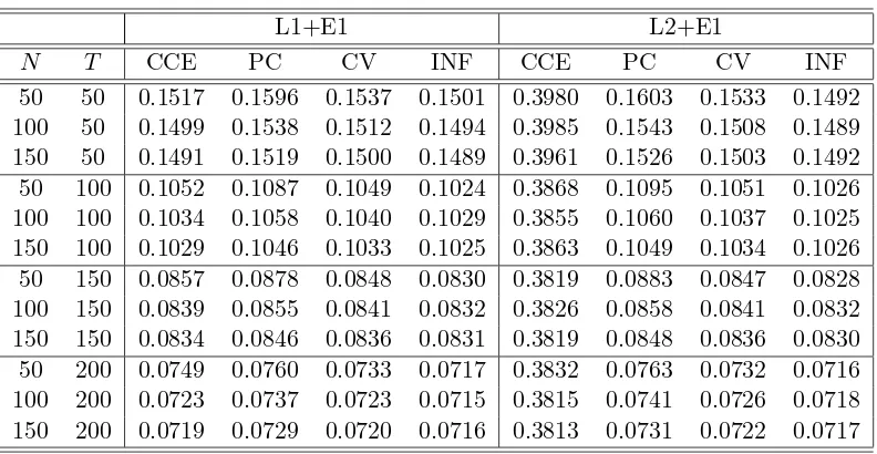
Tables 2-3 report the performance of the CCE, PC, CV and infeasible GLS (denoted by INF) estimators under different loading and error choices in the basic model. In summary, we see that the CCE estimator performs well under L1, but poorly under L2; the PC estimator performs well under E1, but poorly under E2; the CV estimator performs well under all setups.
[image:18.612.109.505.407.612.2]First consider the different loading choices. Under L1, the performance of the CCE estimator is considerably good and very close to that of the CV estimator. The performance of these two estimators is only slightly inferior to the infeasible GLS estimator regardless of homoscedasticity or heteroscedasticity. However, under L2 the performance of the CCE estimator is poor. Not only does it have a large average RMSE, but it also exhibits a slowly decreasing rate for the average RMSE. In contrast, the CV estimator performs closely with the infeasible GLS estimator. The average RMSE of the CV estimator decreases almost at the same speed with that of the infeasible estimator.
Table 2: The performance of the four estimators in the basic model
L1+E1 L2+E1
N T CCE PC CV INF CCE PC CV INF 50 50 0.1517 0.1596 0.1537 0.1501 0.3980 0.1603 0.1533 0.1492 100 50 0.1499 0.1538 0.1512 0.1494 0.3985 0.1543 0.1508 0.1489 150 50 0.1491 0.1519 0.1500 0.1489 0.3961 0.1526 0.1503 0.1492 50 100 0.1052 0.1087 0.1049 0.1024 0.3868 0.1095 0.1051 0.1026 100 100 0.1034 0.1058 0.1040 0.1029 0.3855 0.1060 0.1037 0.1025 150 100 0.1029 0.1046 0.1033 0.1025 0.3863 0.1049 0.1034 0.1026 50 150 0.0857 0.0878 0.0848 0.0830 0.3819 0.0883 0.0847 0.0828 100 150 0.0839 0.0855 0.0841 0.0832 0.3826 0.0858 0.0841 0.0832 150 150 0.0834 0.0846 0.0836 0.0831 0.3819 0.0848 0.0836 0.0830 50 200 0.0749 0.0760 0.0733 0.0717 0.3832 0.0763 0.0732 0.0716 100 200 0.0723 0.0737 0.0723 0.0715 0.3815 0.0741 0.0726 0.0718 150 200 0.0719 0.0729 0.0720 0.0716 0.3813 0.0731 0.0722 0.0717
The reason for the different performance of the CCE estimator under different loading sets is that the space spanned by ˜zt = N1 PNi=1z˙it with ˙zit = ( ˙yit,x˙′it)′ provides a good approximation to the space spanned by ft under L1, but a poor approximation under L2. To see this point more clearly, consider (2.1), which can be written as ˙zit = Λ′ift+ ˙uit. Taking the average overi, we have ˜zt= ˜Λ′f
t+ ˜ut, where ˜Λ and ˜utare defined similarly to ˜
invertible when N goes to infinity②
. The loadings in L1 satisfy these two conditions, but the loadings in L2 violate the first one. In fact, the terms ˜Λ′ft and ˜ut are of the same magnitude under L2. So a good approximation fails. There are cases in which the second condition breaks down. For example, if all rows of Λ share the same mean, then ˜Λ is of rank one asymptotically, which in turn leads to ˜Λ′Λ being singular asymptotically. The˜ simulation results confirm that the CCE estimator performs poorly in this case.
[image:19.612.108.505.358.560.2]Consider then the different choices of the errors. Table 3 shows that the PC estimator performs poorly in the presence of cross-sectional heteroscedasticity (E2). In addition, we find that the performance of the PC estimator is improved marginally under E1, but significantly under E2, whenN becomes larger. According to the theory of Song (2013), the PC estimate is√T-consistent, implying that the performance of the PC estimator should be closely related to T and loosely related to N. This theoretical result is supported by Table 2 but contradicted in Table 3. We think that the underlying reason is due to the computation problem of the minimizer of the objective function in the iterated PC method, as mentioned in Section 1. The extent of this problem depends on the strength of heteroscedasticity. In our simulation, we generate heavy heteroscedasticity, which magnifies the computational problem of the iterated PC method. ③
Table 3: The performance of the four estimators in the basic model
L1+E2 L2+E2
N T CCE PC CV INF CCE PC CV INF 50 50 0.3505 3.4677 0.3667 0.3581 0.4079 2.2194 0.2456 0.2377 100 50 0.3426 2.7550 0.3592 0.3545 0.4084 1.6894 0.2390 0.2362 150 50 0.3470 2.6504 0.3569 0.3543 0.4128 1.2141 0.2382 0.2363 50 100 0.2515 2.8863 0.2494 0.2427 0.3870 2.0866 0.1672 0.1630 100 100 0.2380 2.5816 0.2430 0.2399 0.3856 1.5579 0.1630 0.1616 150 100 0.2417 2.6489 0.2447 0.2430 0.3864 0.9734 0.1644 0.1630 50 150 0.2141 2.9851 0.2008 0.1956 0.3773 1.9264 0.1333 0.1302 100 150 0.2029 2.7919 0.1996 0.1977 0.3804 1.4195 0.1340 0.1326 150 150 0.1973 2.4904 0.1988 0.1973 0.3791 1.0475 0.1319 0.1310 50 200 0.1944 3.5289 0.1763 0.1718 0.3769 1.8067 0.1168 0.1141 100 200 0.1781 3.0194 0.1715 0.1694 0.3787 1.1939 0.1142 0.1131 150 200 0.1726 2.4151 0.1717 0.1705 0.3771 0.8777 0.1128 0.1122
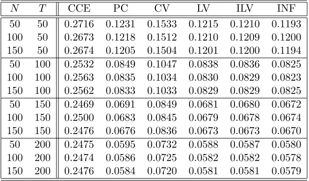
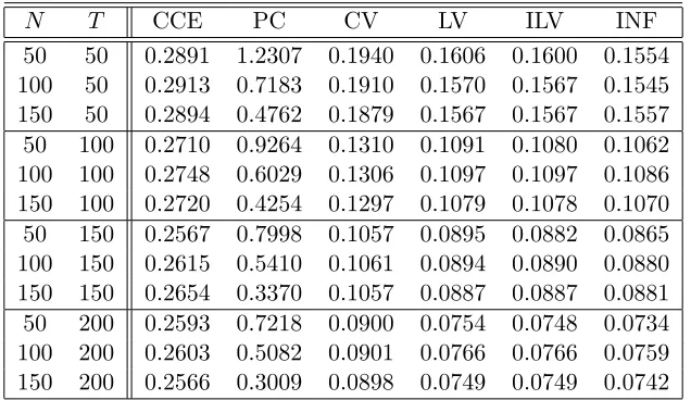
Tables 4-7 report the simulation results for the models with zero restrictions and het-erogeneous coefficients. Overall, these tables reaffirm the result that the CCE estimator performs poorly under L2, and the PC estimator performs poorly under E2. Besides this re-sult, there are several additional points worth noting. First, the CCE and CV estimators are
②
The rank condition in Pesaran (2006) is a necessary but not sufficient condition for invertibility of ˜Λ˜Λ′.
③
inefficient. Under the L1+E1 setup, even whenN and T are large, sayN = 150, T = 200, the average RMSEs of these two estimators are considerably larger than the remaining four estimators. This is not surprising since the two estimation methods do not use the infor-mation contained in the zero restrictions; see the discussion in Section 5. Second, several iterations over the LV estimator indeed improve the finite sample performance, especially whenN andT are small or moderate. In all combinations ofN and T, the ILV estimator outperforms the LV one. Third, under homoscedasticity, the PC, LV and ILV estimators are seen to be efficient since their performance is very close to that of the infeasible GLS estimator, especially when N and T are large.
Table 4: The performance of the six estimators under M2+L1+E1
N T CCE PC CV LV ILV INF 50 50 0.1486 0.0811 0.1527 0.0891 0.0822 0.0790 100 50 0.1483 0.0797 0.1503 0.0868 0.0808 0.0787 150 50 0.1488 0.0792 0.1501 0.0862 0.0803 0.0785 50 100 0.1023 0.0560 0.1046 0.0588 0.0564 0.0546 100 100 0.1026 0.0552 0.1039 0.0575 0.0555 0.0545 150 100 0.1024 0.0549 0.1032 0.0571 0.0552 0.0545 50 150 0.0831 0.0454 0.0849 0.0470 0.0456 0.0443 100 150 0.0831 0.0449 0.0840 0.0463 0.0450 0.0443 150 150 0.0828 0.0445 0.0834 0.0457 0.0447 0.0442 50 200 0.0718 0.0391 0.0732 0.0404 0.0392 0.0382 100 200 0.0717 0.0387 0.0725 0.0396 0.0388 0.0382 150 200 0.0715 0.0384 0.0720 0.0392 0.0385 0.0381
Table 5: The performance of the six estimators under M2+L2+E1
[image:20.612.149.464.455.640.2]Table 6: The performance of the six estimators under under M2+L1+E2
N T CCE PC CV LV ILV INF 50 50 0.2794 0.7402 0.3002 0.2293 0.2172 0.2103 100 50 0.2905 0.2507 0.3020 0.2223 0.2130 0.2081 150 50 0.2980 0.3511 0.3053 0.2282 0.2201 0.2159 50 100 0.2017 0.5204 0.2100 0.1531 0.1495 0.1462 100 100 0.1993 0.1610 0.2081 0.1517 0.1487 0.1468 150 100 0.2057 0.1871 0.2112 0.1524 0.1496 0.1481 50 150 0.1665 0.4558 0.1727 0.1220 0.1198 0.1170 100 150 0.1645 0.3249 0.1675 0.1196 0.1180 0.1166 150 150 0.1641 0.1282 0.1669 0.1202 0.1184 0.1174 50 200 0.1463 0.3222 0.1461 0.1064 0.1048 0.1027 100 200 0.1462 0.1510 0.1484 0.1050 0.1039 0.1027 150 200 0.1447 0.1128 0.1472 0.1043 0.1032 0.1023
Table 7: The performance of the six estimators under under M2+L2+E2
N T CCE PC CV LV ILV INF 50 50 0.2891 1.2307 0.1940 0.1606 0.1600 0.1554 100 50 0.2913 0.7183 0.1910 0.1570 0.1567 0.1545 150 50 0.2894 0.4762 0.1879 0.1567 0.1567 0.1557 50 100 0.2710 0.9264 0.1310 0.1091 0.1080 0.1062 100 100 0.2748 0.6029 0.1306 0.1097 0.1097 0.1086 150 100 0.2720 0.4254 0.1297 0.1079 0.1078 0.1070 50 150 0.2567 0.7998 0.1057 0.0895 0.0882 0.0865 100 150 0.2615 0.5410 0.1061 0.0894 0.0890 0.0880 150 150 0.2654 0.3370 0.1057 0.0887 0.0887 0.0881 50 200 0.2593 0.7218 0.0900 0.0754 0.0748 0.0734 100 200 0.2603 0.5082 0.0901 0.0766 0.0766 0.0759 150 200 0.2566 0.3009 0.0898 0.0749 0.0749 0.0742
7.3 Homogeneous coefficient
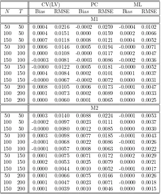
[image:21.612.148.466.323.507.2]Table 8: The performance of the CV(LV), PC and ML estimators under L2+E2+C2
CV(LV) PC ML
N T Bias RMSE Bias RMSE Bias RMSE M1
50 50 0.0004 0.0216 -0.0002 0.0259 -0.0004 0.0102 100 50 0.0004 0.0151 0.0000 0.0159 0.0002 0.0066 150 50 0.0007 0.0118 0.0008 0.0121 0.0004 0.0052 50 100 0.0006 0.0146 0.0005 0.0194 -0.0000 0.0071 100 100 0.0000 0.0108 -0.0000 0.0117 0.0002 0.0047 150 100 -0.0003 0.0081 -0.0003 0.0086 -0.0002 0.0036 50 150 -0.0000 0.0122 0.0005 0.0181 -0.0000 0.0052 100 150 0.0004 0.0084 0.0002 0.0101 0.0001 0.0037 150 150 -0.0000 0.0067 -0.0002 0.0072 0.0000 0.0031 50 200 0.0008 0.0105 0.0006 0.0173 -0.0001 0.0047 100 200 0.0001 0.0073 0.0002 0.0089 0.0000 0.0033 150 200 0.0000 0.0060 0.0001 0.0065 0.0000 0.0025
M2
50 50 0.0003 0.0140 0.0088 0.0224 -0.0001 0.0053 100 50 -0.0002 0.0097 0.0023 0.0111 0.0000 0.0037 150 50 -0.0000 0.0080 0.0012 0.0085 0.0000 0.0030 50 100 0.0003 0.0098 0.0077 0.0185 -0.0001 0.0043 100 100 -0.0001 0.0068 0.0022 0.0086 -0.0001 0.0026 150 100 -0.0001 0.0057 0.0008 0.0063 0.0000 0.0022 50 150 0.0001 0.0075 0.0071 0.0172 0.0002 0.0029 100 150 0.0002 0.0053 0.0025 0.0079 0.0000 0.0021 150 150 0.0000 0.0044 0.0010 0.0052 -0.0001 0.0017 50 200 0.0001 0.0066 0.0075 0.0166 0.0000 0.0026 100 200 0.0001 0.0047 0.0023 0.0071 -0.0000 0.0018 150 200 0.0001 0.0039 0.0010 0.0046 0.0000 0.0015
8
Conclusion
This paper considers the estimation of heterogeneous coefficients in panel data models with common shocks. We propose a two-step method to estimate heterogeneous coefficients, in which the ML method is first used to estimate the loadings and variances of the idiosyn-cratic errors in a pure factor model, and heterogeneous coefficients are then estimated based on the estimates and structural relations implied by the model. Asymptotic prop-erties of the proposed estimators including the asymptotic representations and limiting distributions are investigated and provided.
The proposed estimators are asymptotically efficient in the sense that they have the same limiting distributions as the infeasible GLS estimators. Monte Carlo simulations confirm our theoretical results and show encouraging evidence that the two-step estimators perform robustly in all data setups.
References
Ahn, S. C., and Horenstein, A. R. (2013). Eigenvalue ratio test for the number of factors.
Econometrica, 81(3), 1203-1227.
Bai, J. (2003). Inferential theory for factor models of large dimensions.Econometrica, 71(1), 135-171.
Bai, J. (2009). Panel data models with interactive fixed effects.Econometrica, 77(4), 1229– 1279.
Bai, J. and Li, K. (2012a). Statistical analysis of factor models of high dimension, The Annals of Statistics, 40(1), 436–465.
Bai, J. and Li, K. (2012b). Maximum likelihood estimation and inference of approximate factor mdoels of high dimension, Manuscipt.
Bai, J. and Li, K. (2014). Theory and methods of panel data models with interactive effects,
The Annals of Statistics, 42(1), 142–170.
Bai, J. and Ng, S. (2002). Determining the number of factors in approximate factor models.
Econometrica, 70(1), 191-221.
Chamberlain, G. and Rothschild, M. (1983). Arbitrage, factor structure, and mean-variance analysis on large asset markets,Econometrica,51:5, 1281–1304.
Doz, C., Giannone, D., and Reichlin, L. (2012). A quasi maximum likelihood approach for large approximate dynamic factor models. Review of Economics and Statistics, 94, 1014-1024.
Geweke, John. (1977). The dynamic factor analysis of economic time series, in Dennis J. Aigner and Arthur S. Goldberger (eds.) Latent Variables in Socio-Economic Models (Amsterdam: North-Holland).
Kapetanios, G., Pesaran, M. H., and Yamagata, T. (2011). Panels with non-stationary multifactor error structures. Journal of Econometrics, 160(2), 326-348.
Li, H., Li, Q. and Shi, Y. (2014). Determining the number of factors when the number of factors can increase with sample size. Manuscript.
Onatski, A. (2009). Testing hypotheses about the number of factors in large factor models.
Econometrica, 77(5), 1447-1479.
Pesaran, M. H. (2006). Estimation and inference in large heterogeneous panels with a multifactor error structure, Econometrica, 74(4), 967–1012.
Ross, S. A. (1976). The arbitrage theory of capital asset pricing, Journal of Economic Theory,13(3), 341–360.
Sargent, T. J., and Sims, C. A. (1977). Business cycle modeling without pretending to have too much a priori economic theory. New methods in business cycle research, 1, 145-168.
Stock, J. H., and Watson, M. W. (1998). Diffusion indexes (No. w6702).National Bureau of Economic Research.
Song, M. (2013). Asymptotic theory for dynamic heterogeneous panels with cross-sectional dependence and its applications.Manuscipt, Columbia University.
Appendix A: Proof of Theorem 3.1
Throughout the appendix, we useC to denote a generic finite constant large enough, which need not to be the same at each appearance. In addition, we introduce following notations for ease of exposition.
H= (Λ′Ψ−1Λ)−1; Hˆ = (ˆΛ′Ψˆ−1Λ)ˆ −1; R=MffΛ′Ψˆ−1Λ(ˆˆ Λ′Ψˆ−1Λ)ˆ −1.
We first show thatR=Op(1). The following lemma is useful.
Lemma A.1 Under Assumptions A-D,
(a) R =kN1/2Hˆ1/2k ·Op(1)
(b) R′Mff−11 T
T
X
t=1
ftu′tΨˆ−1Λ ˆˆH=kN1/2Hˆ1/2k2·Op(T−1/2)
(c) ˆHΛˆ′Ψˆ−1h1
T
T
X
t=1
(utu′t−Ψ)
i
ˆ
Ψ−1Λ ˆˆH=kN1/2Hˆ1/2k2·Op(T−1/2)
(d) ˆHΛˆ′Ψˆ−1( ˆΨ−Ψ) ˆΨ−1Λ ˆˆH=kN1/2Hˆ1/2k2·o
p
1
N
N
X
i=1
kΣˆii−Σiik21/2
Proof of Lemma A.1: Consider (a). By the definition of R and ˆH, we have
R=MffΛ′Ψˆ−1Λ(ˆˆ Λ′Ψˆ−1Λ)ˆ −1 =Mff(Λ′Ψˆ−1Λ ˆˆH1/2) ˆH1/2
By the Cauchy-Schwarz inequality,
Λ′Ψˆ−1Λ ˆˆH1/2 =
N
X
i=1
ΛiΣˆ−ii1Λˆ′iHˆ1/2
≤
XN
i=1
ΛiΣˆ
−1/2
ii k2
1/2XN
i=1
kΣˆ−ii1/2Λˆi′Hˆ1/2k21/2
However,
N
X
i=1
kΣˆ−ii1/2Λˆ′iHˆ1/2k2= tr
N
X
i=1
ˆ
H1/2ΛˆiΣˆii−1Λˆ′iHˆ1/2
= trˆ
H1/2Hˆ−1Hˆ1/2
=r (A.1)
Given (A.1), together with the boundedness of ˆΣ−ii1/2 and Λi, we have
Λ′Ψˆ−1Λ ˆˆH1/2
=Op(N1/2)
Then (a) follows.
Consider (b). We first show
1
T
T
X
t=1
u′tΨˆ−1Λ ˆˆH = 1
T
N
X
i=1
T
X
t=1
ftu′itΣˆii−1Λˆ′iHˆ =kN1/2Hˆ1/2k ·Op(T−1/2) (A.2)
By the Cauchy-Schwarz inequality,
1
T
N
X
i=1
T
X
t=1
ftu′itΣˆ−ii1Λˆ′iHˆ ≤C1 N
N
X
i=1
1
T
T
X
t=1
ftu′it
21/2
×
N
X
i=1