Excess Reserves, Monetary Policy and Financial Volatility

Munich Personal RePEc Archive

Excess Reserves, Monetary Policy and

Financial Volatility

Primus, Keyra

University of Manchester

October 2013

Online at

https://mpra.ub.uni-muenchen.de/51670/

Excess Reserves, Monetary Policy and Financial Volatility

Keyra Primus

University of Manchester

Abstract

This paper examines the …nancial and real e¤ects of excess reserves in a New Keyne-sian Dynamic Stochastic General Equilibrium (DSGE) model with monopoly banking, credit market imperfections and a cost channel. The model explicitly accounts for the fact that banks hold excess reserves and they incur costs in holding these assets. Simulations of a shock to required reserves show that although raising reserve require-ments is successful in sterilizing excess reserves, it creates a procyclical e¤ect for real economic activity. This result implies that …nancial stability may come at a cost of macroeconomic stability. The …ndings also indicate that using an augmented Taylor rule in which the policy interest rate is adjusted in response to changes in excess re-serves reduces volatility in output and in‡ation but increases ‡uctuations in …nancial variables. To the contrary, using a countercyclical reserve requirement rule helps to mitigate ‡uctuations in excess reserves, but increases volatility in real variables.

JEL Classi…cation Numbers: E43, E52, E58

Keywords: Excess Reserves, Reserve Requirements, Countercyclical Rule

Contents

1 Introduction 3

2 The Model 8

2.1 Households . . . 9

2.2 Final Good-Producing Firm . . . 11

2.3 Intermediate Good-Producing Firms . . . 11

2.4 Capital Good Producer . . . 13

2.5 Commercial Bank . . . 15

2.6 Central Bank . . . 18

2.7 Government . . . 19

3 Symmetric Equilibrium 20 4 Steady-State and Log-Linearization 21 5 Calibration 22 6 Policy Analysis 25 6.1 Negative Supply Shock . . . 25

6.2 Monetary Policy Shocks . . . 27

6.2.1 Increase in Re…nance Rate . . . 27

6.2.2 Increase in Reserve Requirement Ratio . . . 28

6.3 Liquidity Shock: Increase in Bank Deposits . . . 31

6.4 Simultaneous Shocks to Deposits and Reserve Requirements . . . 32

7 Policy Rules for Managing Excess Reserves 33 7.1 An Augmented Taylor Rule . . . 33

7.2 A Countercyclical Reserve Requirement Rule . . . 36

8 Conclusion 38

References 40

Appendix A: Solutions to Optimization Problems 46

Appendix B: Steady-State Equations 50

Appendix C: Log-Linearized Equations 54

1

Introduction

Excess reserves have been a common feature of the banking system of many countries across the world.1 _{In developed countries, the phenomenon of excess reserves has become more}

apparent since the global …nancial crisis. For instance, in the case of the United States, the sharp increase in excess reserves since 2008 occurred because risk averse banks stopped lending to each other and engaged in liquidity hoarding (see Ashcraft et al. (2009), Hilton and McAndrews (2010) and Jenkins (2010)). Others argued that the policy initiatives undertaken by the Federal Reserve in response to the crisis caused the quantity of bank reserves to surge (see Keister and McAndrews (2009) and Ennis and Wolman (2012)). Similarly, excess reserves have been growing rapidly in commercial banks in the Euro Area since the onset of the global economic crisis (see European Central Bank (2008) and Sol Murta and Garcia (2009)).

In developing economies, the problem of excess reserves is more prevalent. For several years, the banking system of some developing countries has recorded high persistent liq-uidity. For instance, Figure 1 shows the excess liquidity situation in three small developing countries. Inspection of the data reveals that excess reserves have been greater than 15 percent for most of the period in Belize and Trinidad and Tobago, and above 25 percent in Jamaica. Given its importance to the monetary transmission process, several researchers have empirically examined the determinants of excess liquidity in developing economies. Contributions along these lines include Maynard and Moore (2005) for Barbados, Saxe-gaard (2006) for Sub-Saharan Africa, Khemraj (2007, 2009) for Guyana, Anderson-Reid (2011) for Jamaica, Pontes and Sol Murta (2012) for Cape Verde, Jordan et al. (2012) for The Bahamas and Primus et al. (forthcoming) for Trinidad and Tobago. In most cases, these studies show that excess reserves appear to be a structural phenomenon.2

As highlighted in Agénor and El Aynaoui (2010), the reasons for excess liquidity can be categorised into structural and cyclical factors. One structural factor is a low degree of

1_{In most …nancial systems, excess liquidity refers to the maintenance by banks of a higher level of funds}

than is normally required to meet their statutory reserve requirements and settlement balances. Excess liquidity (or excess reserves) is measured as the di¤erence between total bank reserves and required bank reserves. For this reason, the terms excess liquidity and excess reserves are used interchangeably in the literature.

2_{Excess bank liquidity is also a problem for large developing countries, such as Brazil, Russia, India,}

…nancial development. Therefore, excess liquidity tends to be more persistent in countries with underdeveloped …nancial markets, such as ine¢cient payment systems, or an under-developed market for government securities (see Saxegaard (2006)). Another structural factor is a high degree of risk aversion. In an environment of increased uncertainty, risk averse banks charge a high risk premia to reduce demand for loans and to safeguard their loan portfolio. This leads to a voluntary build-up of excess liquid assets.3

Regarding the cyclical factors, one of the main sources of excess reserves is foreign currency in‡ows (Heenan (2005) and Ganley (2004)). Current account in‡ows arise mainly through revenues received from commodity exports. Therefore, exporters of minerals, such as Botswana, and oil exporting economies, such as Nigeria and Trinidad and Tobago, observe huge surpluses in their current account when commodity prices are high on world markets. Particularly in oil-producing countries, a rise in oil prices results in an increase in government revenues. In many cases, these energy windfalls are used to …nance an increase in government spending. As a result, the banking system of these economies holds large quantities of involuntary excess liquidity.4 Capital account in‡ows may arise from aid-related transfers, foreign direct investment and portfolio in‡ows. Another cyclical cause of excess liquidity is in‡ation. Because in‡ation leads to higher volatility in relative prices and an increase in riskiness of investment projects, it raises uncertainty about the value of collateral. This causes banks to demand a higher risk premium, which increases the lending rate. The higher loan rate can lead to a contraction in credit demand and increase excess reserves.

In an attempt to withdraw excess liquidity from the …nancial system, central banks have used open market operations, and issued central bank bills.5 _{Central banks have also issued}

long-term securities (bonds) and implemented special deposit facilities. In addition, reserve requirements6 _{have been used frequently to manage liquidity.}7 _{For instance, between 2006}

3_{Similarly, in a crisis environment where banks perceive an increase in the risk of default on loans, they}

may be unwilling to lend. For instance, Agénor et al. (2004) found that the contraction in bank credit and the associated increase in excess reserves in Thailand following the Asian …nancial crisis in the late 1990s resulted from supply related factors, which emanated from the banks.

4_{According to Agénor and El Aynaoui (2010, p. 923), involuntary excess liquidity is "the involuntary}

accumulation of liquid reserves by commercial banks". Several researchers have examined the issue of involuntary excess liquidity. See for instance, Saxegaard (2006), Bathaluddin et al. (2012) and Primus et al. (forthcoming).

5_{See Nyawata (2012) for a discussion of the pros and cons of using treasury bills and central bank bills}

to absorb liquidity.

6_{Reserve requirement levels vary greatly across countries. It has been observed that these ratios are}

generally higher in developing countries, when compared to developed countries (see Appendix D).

and 2009, the central banks of China, India and Trinidad and Tobago have all increased reserve requirements to mop up excess liquidity. Using reserve requirements can help the central bank or the government to reduce the quantity of excess reserves in the …nancial system without incurring interest costs, which are associated with the issuance of securities (Gray (2011)). Also, reserve requirements can be more e¤ective because selling securities to sterilize excess liquidity can in fact be self-defeating as it can cause market interest rates to increase and stimulate capital in‡ows, thereby making the excess liquidity problem worse if to begin with it resulted from large in‡ows (Lee (1997)). One disadvantage to note however is reserve requirements act as a tax on the …nancial sector (Central Bank of Trinidad and Tobago (2005) and Montoro and Moreno (2011)).

In the presence of excess liquidity, the e¤ectiveness of monetary policy can be limited or asymmetric. As empirically documented in Lebedinski (2007) for Morocco, when banks hold excess reserves they are more likely to respond in an asymmetric manner when adjust-ing deposit rates. Therefore, followadjust-ing an increase in the re…nance rate or a reduction in the required reserve ratio, banks may not raise deposit rates. As a result, a contractionary monetary policy may be less e¤ective in reducing in‡ation (Agénor and El Aynaoui (2010)). Furthermore, when banks hold excess liquidity, an expansionary monetary policy may not be successful in stimulating bank credit.8

Despite the impact excess reserves can have on the transmission mechanism of monetary policy, there have been few attempts to examine the role of reserves in a New Keynesian general equilibrium framework.9 This paper contributes to the existing literature by ex-plicitly modeling excess reserves in a Dynamic Stochastic General Equilibrium (DSGE) framework with monopoly banking, credit market imperfections and a cost channel. The model extends and modi…es the framework in Agénor and Alper (2012), and integrates aspects of Agénor et al. (2013) and Glocker and Towbin (2012). In this framework, the bank holds excess reserves and there are convex costs associated with holding these re-serves as in Glocker and Towbin (2012). The central bank sets its policy interest rate, using a Taylor-type rule. Therefore, this framework can be applied to other high- and

tool. See Montoro and Moreno (2011), Robitaille (2011) and Tovar et al. (2012) for further discussions.

8_{This is particularly important when banks hold excess reserves for precautionary purposes. In this case,}

an expansionary monetary policy will only raise the amount of excess reserves further, and will not help to expand credit.

9_{Christiano et al. (2010) and Samake (2010) incorporated excess reserves into a general equilibrium}

middle-income countries, where the …nancial system is su¢ciently developed so monetary policy can operate through the manipulation of a short-term interest rate.

The model is used to examine the …nancial and real e¤ects of a productivity shock, an increase in the policy interest rate, a shock to the reserve requirement ratio and an exogenous increase in bank liquidity. Also, simultaneous shocks are applied to deposits and reserve requirements to examine whether increasing required reserves in response to a surge in liquidity is an e¤ective measure. This experiment is one of the key contributions to this paper. Although it has been often observed in practice that raising reserve requirements can indeed o¤set an increase in liquidity, this is the …rst attempt to model this in a New Keynesian general equilibrium framework. In addition, we investigate the responses of the variables in the model following a liquidity shock when two alternative policy rules are used: an augmented Taylor rule in which the central bank adjusts its policy rate in response to changes in excess reserves, and a countercyclical rule in which the reserve requirement ratio reacts to deviations in excess reserves.

The model is calibrated based on Trinidad and Tobago data due to the fact that excess reserves have been growing very rapidly in that country. The results show that a negative supply shock and a contractionary monetary shock have the traditional e¤ects. In the former case prices increase and output declines, while in the latter both in‡ation and output fall. As the re…nance rate rises following both types of shocks, the opportunity cost of holding excess reserves increases. The …ndings also indicate that although a positive shock to required reserves is successful in reducing excess reserves, the e¤ect is expansionary for real economic activity. In the case of a liquidity shock, a simultaneous increase in reserve requirements can assist in reducing the quantity of excess reserves in the …nancial system. Furthermore, when an augmented Taylor rule which includes excess reserves is used, a liquidity shock has a less dampening e¤ect on real variables but increases ‡uctuations in …nancial variables. To the contrary, using a countercyclical reserve requirement rule has the opposite e¤ect for both real and …nancial variables.

Figure 1. The Percent of Excess Reserves to Total Reserves in Various Countries10

Source: Central Bank of Belize.

Source: Central Bank of Trinidad and Tobago.

Source: Bank of Jamaica.

1 0_{In the case of Trinidad and Tobago, prior to January 2006 excess liquidity is measured by commercial}

2

The Model

Consider an economy which contains seven classes of agents: identical in…nitely-lived house-holds indexed byh2[0;1], a …nal producing …rm, a continuum of intermediate good-producing …rms indexed byj2[0;1], a capital good producer, a commercial bank (a bank, for short), the central bank (whose responsibility is to regulate the commercial bank) and the government.

Households consume and supply labour to intermediate good-producing …rms. House-holds also choose the real levels of cash, deposits and government bonds to hold at the be-ginning of the period. Each household supplies labour to the intermediate good-producing …rm which it owns. Intermediate good-producing …rms use the labour provided by house-holds and capital (which is rented from the capital good producer) to produce a unique good that is sold on the monopolistically competitive market. The pricing mechanism of Rotemberg (1982) is used to account for the fact that intermediate good-producing …rms incur a cost in adjusting prices. The …nal good-producing …rm aggregates imperfectly substitutable intermediate goods into a single …nal good which is used for consumption, investment or government spending. The …nal good is sold at a perfectly competitive price. The capital good producer purchases the …nal good for investment and combines it with existing capital stock to produce new capital goods. In this model, wages are fully ‡exible and adjust to clear the market.

The commercial bank, which is owned by households, supplies credit in advance to in-termediate good-producing …rms to …nance their short-term working capital needs. Owing to the fact that these loans are short-term in nature, we assume that they do not carry any risk. The bank also supplies credit to the capital good producer for investment …nancing. The bank’s supply of loans is perfectly elastic at the prevailing lending rate. These loans are extended prior to production or investment and are repaid at the end of the period. The bank pays interest on household deposits and central bank loans. In addition, the bank is required to hold minimum reserves against deposits at the central bank, and it has an explicit demand for excess reserves. Total reserves at the central bank are remunerated at the reserve rate denoted byiM

t . The bank determines the total reserve ratio, the deposit

in reserve management models.11 _{Therefore, increased uncertainty about the size of cash}

withdrawals does not in‡uence the quantity of excess bank reserves in this model.

2.1 Households

Each household, h, chooses consumption, labour supply to intermediate good-producing …rms and real monetary assets. The objective of a representative household is to maximize the following utility function,

U =Et

1

X

t=0

t[Cht]1

1

1 1 + Nln(1 Nht) + XlnXht; (1)

whereChtis household consumption,Nhtis the share of total time endowment (normalized

to unity) household h spent working, Xht is a composite index of real monetary assets,

> 0 gives the intertemporal elasticity of substitution in consumption, _N; _X > 0 are preference parameters with respect to leisure and money holdings respectively, 2 (0;1)

is the discount factor and Et is the expectation operator conditional on the information

available at the beginning of periodt.

The composite monetary asset is a combination of real cash balancesM_htH and real bank depositsDht, which can be represented by the following Cobb-Douglas function,

Xht= (MhtH) Dht1 ; (2)

where 2(0;1).

Real wealth of household h at the end of periodt,Aht, is given by,

Aht=MhtH +Dht+BhtH; (3)

whereBH

ht denotes holdings of one-period real government bonds.

At the beginning of period t, each household enters with MH

ht 1 level of cash. Holding

money balances yield no return, while deposits and government bonds yield gross returns of(1+iD

t )and(1+iBt ), respectively. Therefore, the total real returns from holding deposits

and government bonds from period t 1, adjusted for the rate of in‡ation, are denoted respectively by(1 +iD_{t 1})Dht 1P_Pt_t1 and(1 +iBt 1)BhtH 1

Pt 1

Pt , wherePtrepresents the price

of the …nal good.

In addition, households supply labour to intermediate good-producing …rms, for which they receive a total real factor payment !tNht, where !t denotes the economy-wide real

1 1_{In reserve management models, optimal reserves are a function of deposit ‡uctuations (see Morrison}

wage. Each household owns an intermediate good-producing …rm so all the pro…ts made by that …rm, JI

ht, are paid to the respective household. Also, each household receives a

…xed fraction'_h 2(0;1)of the bank’s pro…ts,J_tB, and the capital good producer’s pro…ts,

J_tK, withR₀1'_hdh= 1. Each household is also required to pay a lump-sum tax, whose real value isTht.

The real budget constraint of householdh is,

M_htH +Dht+BhtH !tNht Tht+MhtH 1(

Pt 1

Pt

) + (1 +iD_{t 1})Dht 1(

Pt 1

Pt

) (4)

+(1 +iB_{t 1})B_htH ₁(Pt 1

Pt

) +J_htI +'_hJ_tB+J_tK Cht:

Each household maximizes lifetime utility with respect toCht,Nht,MhtH,Dht andBhtH,

takingiD_t ,iB_t ,Pt, andTht as given. Maximizing (1) subject to (4) yields the following …rst

order conditions,12

C_ht1= = Et (Cht+1) 1= (

1 +iB_t

1 + t+1

) ; (5)

Nht= 1 N

(Cht)1=

!t

; (6)

M_htH = X (Cht)

1= _{(1 +i}B t )

iB t

; (7)

Dht= X

(1 )(Cht)1= (1 +iBt )

iB t iDt

; (8)

where t+1 = (Pt+1 Pt)=Pt is the in‡ation rate. The transversality condition is

deter-mined by the following equation,

lim

s!1Et+s t+s

s_(MH

t+s) = 0: (9)

Equation (5) is the standard Euler equation which describes the optimal consumption path. Equation (6) represents the optimal labour supply which is positively related to the real wage and negatively related to consumption. Equation (7) shows that the demand for real cash balances depends positively on consumption and negatively on the opportunity cost of holding cash (measured by the rate of return on government bonds). Equation (8) denotes the real demand for deposits which is positively related to consumption and the deposit rate, and negatively related to the bond rate.

2.2 Final Good-Producing Firm

The …nal good producer assembles a continuum of imperfectly substitutable intermediate goods Yjt, indexed by j 2 (0;1), to produce the …nal good Yt, which is used for private

consumption, government consumption and investment. The production technology for combining intermediate goods to produce the …nal good is given by the standard Dixit-Stiglitz (1977) technology,

Yt=

Z 1

0

[Yjt]( 1)= dj

=( 1)

; (10)

where >1 represents the elasticity of demand for each intermediate good.

Given the prices of intermediate goods,Pjt, and the …nal good price,Pt, the …nal

good-producing …rm chooses the quantities of intermediate goods to maximize its pro…ts. The pro…t maximization problem of the …nal good producer is given by,

max

Yjt

Pt

Z 1

0

[Yjt]( 1)= dj

=( 1) Z ₁ 0

PjtYjtdj: (11)

The …rst-order condition with respect toYjt is,

Yjt = (

Pjt

Pt

) Yt: (12)

Equation (12) gives the demand for each intermediate goodj. Substituting (12) in (10) and imposing a zero-pro…t condition, the …nal good price is represented by,

Pt=

Z 1

0

(Pjt)1 dj

1=(1 )

: (13)

2.3 Intermediate Good-Producing Firms

Each intermediate good-producing …rm, j, produces a perishable good which is sold on a monopolistically competitive market. To produce these goods, each …rm rents capital at the pricerK_t from the capital good producer and combines it with labour. The technology faced by each intermediate good-producing …rm is given by the Cobb-Douglas production function,

Yjt=AtKjtNjt1 ; (14)

whereNjt is householdh=jlabour hours,Kjt is the amount of capital rented by the …rm,

technology shock which follows a …rst-order autoregressive process, At = AtA1exp At ,

where _A2(0;1)and A_t N(0; A).

In order to pay wages in advance, …rm j takes a loan from the bank at the beginning of the period. The amount borrowed is,

LF;W_jt = W!tNjt; (15)

where LF;W_jt represents the real value of loans demanded by intermediate good producers for allt 0and W 2(0;1). Similar to Agénor et al. (2013), it is assumed that short-term loans for working capital do not carry any risk and are therefore contracted at a rate that re‡ects only the marginal cost of borrowing from the central bank,iR_t, which is the re…nance rate. The wage bill, inclusive of interest payments is (1 +iR_t ) W!tNjt + (1 W)!tNjt.

Rearranging this gives(1+ WiR_t)!tNjt, which shows the …rm’s wage bill includes a constant

share of …nancing of working capital needs. Thus, W indicates the strength of the cost channel; if W = 0, no cost channel exists.

Intermediate good producers solve a two stage problem. In the …rst stage, given input prices, …rms integrate capital and labour in a perfectly competitive market in order to minimize their total costs. The cost minimization problem for …rmj is,

min

Njt;Kjt

(1 + WiR_t)!tNjt+rtKKjt : (16)

Minimizing (16) subject to (14), the …rst-order conditions with respect toNjt andKjt

equate the marginal products of capital and labour to their relative prices, from which the capital-labour ratio is obtained,

Kjt

Njt

= (

1 )[

(1 + WiR_t)!t

rK

t

]: (17)

The unit real marginal cost is,

mcjt =

(1 + W_iR

t)!t 1 (rKt )

(1 )1 _A

t

: (18)

In the second stage, each …rm chooses prices, Pjt, to maximize the discounted real

value of current and future pro…ts. Nominal price stickiness is introduced along the lines of Rotemberg (1982), by assuming that intermediate good-producing …rms incur a cost in adjusting prices. These price adjustment costs, P ACjt, which are measured in terms of

aggregate output, Yt, take the form,

P ACjt = F

2

Pjt

Pjt 1

1

2

where _F 0 is the degree of price stickiness.

Thus, the pro…t maximization problem for the intermediate good producer is,

max

Pjt

Et

1

X

t=0

t

tJjtI; (20)

where t t is the …rm’s discount factor for period t, with t representing the marginal

utility gained from consuming an additional unit of pro…t. Real pro…ts,J_jtI, are de…ned as,

J_jtI =Yjt mcjtYjt P ACjt: (21)

Substituting (12) and (19) in (21) and taking mcjt, Pt and Yt as given, the …rst-order

condition with respect toPjt is,

(1 ) t Pjt

Pt

Yt

Pt

+ tmcjt Pjt

Pt

1

Yt

Pt t F

Pjt

Pjt 1

1 Yt

Pjt 1

(22)

+ _FEt

(

t+1

Pjt+1

Pjt

1 Pjt+1

P2

jt

!

Yt+1

)

= 0:

Equation (22) gives the adjustment process of the nominal pricePjt. When there is no

price adjustment cost ( _F = 0), the price equals a mark-up over the real marginal cost,

Pjt =

1 mcjtPt: (23)

In a symmetric equilibrium Pjt =Pt for allj; hence the real marginal cost equals the

reciprocal of the mark-up,mct= ( 1).

2.4 Capital Good Producer

In the economy, all the capital is owned by the capital good producer who employs a linear production function to produce capital goods. As in Agénor et al. (2013), at the beginning of each period, the capital good producer purchasesItof the …nal good from the …nal good

producer. Because payments for these …nal goods must be made in advance, the capital good producer borrows from the bank,

LF;I_t =It; (24)

The capital good producer combines undepreciated capital from the previous period, with investment to produce new capital goods. New capital goods, denoted as Kt+1, are

given by,

Kt+1 =It+ (1 )Kt K

2

Kt+1

Kt

1

2

Kt; (25)

where Kt = R₀1Kjtdj, 2 (0;1) gives the constant rate of depreciation and K > 0

measures the magnitude of adjustment costs. The capital good producer rents the new capital stock to intermediate good-producing …rms at the raterK

t .

The capital good producer chooses the amount of capital stock in order to maximize the value of the discounted stream of dividend payments to the household. The optimization problem of the capital good producer is given by,

max

Kt+1

Et

1

X

t=0

t

tJtK; (26)

where real pro…ts,JK

t , can be denoted as,

J_tK =rK_t Kt (1 +iLt)It: (27)

Maximizing (26) subject to (25), the …rst-order condition is,

EtrKt+1 = (1 +iLt)Et 1 + K(

Kt+1

Kt

1) ( 1 +i

B t

1 + t+1

) (28)

Et

(

(1 +iL_t+1)

"

(1 ) + K 2 [

Kt+2

Kt+1 2

1]

#)

:

Equation (28) shows the expected rental rate of capital is a function of the current and expected loan rates, the cost of adjusting capital across periods, the bond rate, the depreciation rate and the in‡ation rate. The opportunity cost of investing in physical capital is measured by the real rate of return on government bonds. If the capital good producer does not borrow at the beginning of the period, and there are no adjustment costs( K = 0),

EtrKt+1 =Et(

1 +iB_t

1 + t+1

) 1 + : (29)

2.5 Commercial Bank

The bank receives depositsDtfrom households at the start of each period. These deposits

are used to …nance loans to intermediate good-producing …rms to cover wage payments and to the capital good producer for investment. Therefore, combining (15) and (24), total lending, LF

t, in real terms is,

LF_t = W!tNt+It: (30)

Given households’ deposits and total loans to …rms, to …nance any shortfall in funding, the bank borrows from the central bank,LB_t , for which it pays a net interest rate iR_t.

Assets of the commercial bank at the beginning of periodtconsist of real loans to …rms and real total reserve holdings,T Rt, whereas its liabilities comprise of real loans from the

central bank and real deposits. The bank’s balance sheet is thus,

LF_t +T Rt=LBt +Dt: (31)

Total reserves comprise of excess reserves, ERt, and required reserves,RRt, which are

the compulsory minimum amount of reserves the bank must hold at the central bank. Thus,

T Rt=ERt+RRt; (32)

where total reserves are a portion T R_t of deposits and required reserves are a percent _tof deposits. Therefore, T Rt= T Rt Dt and RRt = tDt; where T Rt , t2(0;1). Using these

in (32), excess reserves are therefore determined residually,13

ERt= ( T Rt t)Dt: (33)

Reserves held at the central bank are remunerated at the rate iM

t ,14 where iMt < iRt .

The bank therefore chooses the total reserve ratio, the deposit rate and the lending rate to maximize its present discounted value of real pro…ts. Hence, the bank’s pro…t maximization problem is,

max

f T R

t ;1+iDt ;1+iLtg

E_t

1

X

t=0

t

tJtB; (34)

1 3_{In principle, the bank should determine directly excess reserves; however, it is more convenient to solve}

for total reserves …rst, and use this solution to determine excess reserves.

1 4_{A few studies have discussed how interest on reserves can be used as a policy instrument (see Goodfriend}

where,E_t is the expectations operator based on information available at the beginning of period t and JB

t represents real bank pro…ts at the end of period t. Therefore, expected

real bank pro…ts can be de…ned as,

E_t J_tB = (1 + WiR_t )LF;W_t +Q_tF(1 +iL_t)LF;I_t + (1 QF_t) CKt (35)

+(1 +iM_t )T Rt (1 +iDt )Dt (1 +iRt )LBt ( T Rt t)Dt;

where C 2(0;1)and QF_t 2(0;1)is the repayment probability.

From equation (35), the …rst term on the right-hand side, (1 + WiR_t)LF;W_t , shows repayment on loans to intermediate good-producing …rms. The second term, QF

t (1 +

iL

t)LF;It , represents expected repayment on loans to the capital good producer, providing

that there is no default. The third term, (1 QF

t ) CKt, denotes the bank’s earnings in

case of default, where 1 QF

t represents the probability of default. This term therefore

shows real e¤ective collateral, given by a fraction C of the real capital stock. The expression (1 +iM_t )T Rt denotes the principal plus interest gained from total reserves,

whereas(1+iD_t )Dtrepresents the principal and interest paid on real deposits, and(1+iRt )LBt

re‡ects the gross repayments to the central bank. Similar to Glocker and Towbin (2012), the …nal term, ( T R_{t t})Dt, is included to represent the convex costs of holding reserves,

which are proportional to the amount of real deposits. Thus,

( _tT R _t) = C1( T Rt t) + ₂C2( T Rt t)2+"Rt: (36)

From equation (36), C1 and C2 are cost function parameters. The linear term,

C1( T Rt t), determines steady-state deviations from the required reserve ratio. A

pos-itive deviation from the ratio may generate small bene…ts because holding excess reserves reduces the costs of liquidity management. Intuitively, if the bank fails to meet the reserve requirement it has to face the penalty rate for funds borrowed from the central bank. The quadratic term, C2

2 ( T Rt t)2, indicates that negative deviations from the required ratio

may generate large costs. For instance, the central bank may impose a higher penalty rate in cases where there are large negative deviations from its target, and at the same time, cease remuneration of excess reserves.15 The last term,"R_t , represents a cost shock.

From the balance sheet constraint (31), and given that LF_t and Dt are determined by

the private agents’ behaviour, borrowing from the central bank can be solved for residually. Therefore, usingT Rt= T Rt Dtin (31) yields,

LB_t =LF_t (1 T R_t )Dt: (37)

Using T Rt = T Rt Dt and substituting (36) and (37) in (35) gives the bank’s static

optimization problem,

max

f T R

t ;1+iDt ;1+iLtg

f(1 + WiR_t )LF;W_t +QF_t (1 +iL_t)LF;I_t + (1 QF_t) CKt (38)

+(1 +iM_t ) T R_t Dt (1 +iDt )Dt (1 +iRt) LFt (1 T Rt )Dt

C1( T Rt t) + C2

2 (

T R

t t)2+"Rt Dtg:

The …rst-order condition with respect to T R t is, T R

t = t+

1 +iM

t + C1 1 +iRt C2

:

The di¤erence between the total reserve ratio and the required reserve ratio T R_{t t}, represents the excess reserve ratio, ER_t , which is given by,

ER t =

1 +iM_t + C1 1 +iRt C2

: (39)

The …rst-order condition with respect to1 +iD t is,

(1 +iM_t ) T R_t ( @Dt

@ 1 +iD_t ) (1 +i

D t )(

@Dt

@ 1 +iD_t ) Dt

+(1 +iR_t )(1 T R_t )( @Dt

@ 1 +iD_t ) ( )(

@Dt

@ 1 +iD_t ) = 0;

using _D = ( @Dt

@(1+iD t )

)((1+i

D t )

Dt ) to represent the constant interest elasticity of the supply of

deposits by the household results in,

1 +iD_t = (1 + 1

D

) 1[(1 +iR_t ) T R_t (iR_t iM_t ) (40)

+ C1( T Rt t) ₂C2( T Rt t)2]:

The …rst-order condition with respect to1 +iL_t is,

QF_tLF;I_t +QF_t (1 +iL_t) @L

F;I t

@(1 +iL_t) (1 +i

R t)

@LF;I_t

@(1 +iL_t) = 0;

using _L= @LF;It

@(1+iL t)

(1+iL t)

LF;It

to denote the interest elasticity of demand for loans for investment yields,

1 +iL_t = 1 +i

R t

Equation (39) represents the bank’s excess reserve ratio. This shows that ER

t increases

with iM

t but falls with iRt. Therefore, the excess reserve ratio is decreasing in the spread

between the interest rate on reserves and the re…nance rate. By holding an additional unit of excess reserves at the central bank, the bank bene…ts by gaining 1 +iM_t ; at the same time, it saves because it does not have to borrow from the central bank to meet reserve requirements. By contrast, the bank also incurs costs for holding the extra unit of excess reserves. Therefore, equation (39) balances the costs and the bene…ts of holding excess reserves. From equation (40), the (gross) interest rate on deposits depends on the marginal cost of borrowing from the central bank, which is lowered in the presence of remunerated reserves by the di¤erence between the re…nance rate and the interest rate on reserves. The deposit rate also depends on the costs associated with holding excess reserves. Equation (41) shows that the (gross) lending rate depends positively on the marginal cost of borrowing from the central bank and negatively on the repayment probability,QF

t.

As in Agénor and Alper (2012), the repayment probability is taken to depend posi-tively on "micro" and "macro" factors, namely, the real e¤ective collateral-loan ratio and economic activity. Therefore,QF_t increases with the collateral provided by …rms and falls with the amount borrowed. Hence,

QF_t = ₀

C_K t

LF;I_t

! 1

Yt

Y

2

; (42)

where ₀; ₁; ₂ > 0 and (Yt=Y) represents the output gap, with Y denoting the

steady-state value of output16 under fully ‡exible prices.

2.6 Central Bank

The central bank’s assets consist of government bonds, BC

t , and loans to the commercial

bank, LB_t , whereas its liabilities consist of total reserves, T R_t, and currency supplied to households and …rms,M_ts. Therefore, the central bank’s balance sheet is given by,

B_tC +LB_t =T R_t+M_ts: (43)

UsingT Rt= T Rt Dt and rearranging, equation (43) becomes,

M_ts =B_tC+LB_t T R_t Dt: (44)

1 6_{Similar to other studies (see, for instance, Meh and Moran (2010)), the output gap is measured in terms}

Equation (44) shows the supply of currency is matched by government bonds and central bank loans extended to the commercial bank, less the fraction of deposits held at the central bank.

In this economy, the central bank sets the policy interest rate using a Taylor-type rule (see Taylor (1993)), and supplies all the liquidity the bank needs through a standing facility. The policy rule is of the form,

iR_t = iR_{t 1}+ (1 )[r+ t+"1( t T) +"2ln

Yt

Y ] + t; (45)

where 2(0;1)measures the degree of interest rate smoothing,r is the steady-state value of the real interest rate on bonds, t represents current in‡ation, T 0 is the central

bank’s in‡ation target,"1; "2>0measure the relative weights on in‡ation deviations from

its target and the output gap, respectively and tis a serially correlated shock with constant

variance, which follows a …rst order autoregressive process of the form,

t= t 1exp ( t); (46)

where 2(0;1)and _t N(0; )is a serially correlated random shock with zero mean. The standard speci…cation (45) will be extended later in the text to include a measure of excess reserves, in order to examine the dynamic e¤ects of an increase in bank reserves under an interest rate rule which reacts directly to changes in liquidity.

2.7 Government

The government purchases the …nal good, collects taxes, and issues one-period risk-free bonds,Bt, which are held by the central bank,BtC, and households, BHt . Total bonds can

be denoted by,Bt=BCt +BHt . The government’s real budget constraint is given by,

Bt+Tt+iRt 1LBt 1

Pt 1

Pt

+iB_{t 1}B_tC₁Pt 1 Pt

iM_{t 1}T Rt 1

Pt 1

Pt

= (47)

Gt+ (1 +iBt 1)Bt 1Pt 1

Pt

;

whereGtdenotes real government spending andTtrepresents real lump-sum tax revenues.

The sum of the terms iR_{t 1}LB_{t 1}Pt 1

Pt , i

B t 1BtC1

Pt 1

Pt and i

M

t 1T Rt 1P_Pt_t1 (adjusted for the

Government purchases represent a constant fraction, 2(0;1), of output of the …nal good,

Gt= Yt: (48)

3

Symmetric Equilibrium

In a symmetric equilibrium, all …rms producing intermediate goods are identical so they produce the same output, and prices are the same across …rms. Also, all households supply the same number of labour hours. Therefore, Kjt =Kt,Njt =Nt, Yjt =Yt,Pjt =Pt, for

allj 2(0;1).

It is necessary for equilibrium conditions in the credit, deposit, goods and cash markets to be satis…ed.17 The supply of loans by the commercial bank and supply of deposits by households are perfectly elastic at the prevailing interest rates; as a result, the markets for loans and deposits always clear. To satisfy equilibrium in the goods markets, production must be equal to aggregate demand. Thus, using (19),

Yt=Ct+Gt+It+ F

2 ( 1 + t

1 + 1)

2_Y

t: (49)

The equilibrium condition of the market for cash is,

M_ts =M_tH +M_tF; (50)

whereMF t =

R1

0 MjtFdj represents the total cash holdings of intermediate good-producing

…rms and the capital producer. It is assumed that bank loans to all …rms are extended in the form of cash such that, LF

t = MtF. Substituting this in (50), Mts = MtH +LFt .

ReplacingMs

t from (44) gives,

B_tC+LB_t T R_t Dt=MtH+LFt: (51)

UsingLB_t from (37) into (51) gives,

BC_t + (LF_t + T R_t Dt Dt) T Rt Dt=MtH +LFt;

or,

BC =M_tH +Dt: (52)

Given that the total stock of bonds held by the central bank is constant, equation (52) implies that real cash balances are inversely related to real bank deposits. This equation also represents the money market equilibrium condition, from which the equilibrium bond rate is obtained.

4

Steady-State and Log-Linearization

This section presents some of the key steady-state and log-linearized equations of the model. Further details on all the steady-state equations are shown in Appendix B, whereas the log-linearized equations are outlined in Appendix C.

Given that the steady-state is characterized by zero in‡ation, from equation (5), the steady-state value of the bond rate (which is equal to the re…nance rate) is given by,

1 +iB = 1 +iR= 1 +r = 1:

The equality between iB _{and i}R _{implies that the commercial bank has no incentive to}

borrow from the central bank in order to buy government bonds. The steady-state deposit and lending rates are given by,

1 +iD = (1 + 1

D

) 1[(1 +iR) T R(iR iM)

+ C1( T R ) C2

2 (

T R ₎2_];

1 +iL= 1 +i

R

QF 1

L + 1

:

In the steady state, the repayment probability is inversely related to the …rm’s asset over its liabilities,

QF = ₀

C_K

LF;I

1

:

The steady-state value of the excess reserve ratio is given by,

ER₌ 1 +iM + C1 (1 +iR) C2

:

In order to solve the model, each variable is log-linearized around a non-stochastic, zero-in‡ation steady-state. The log-linearized deposit rate is denoted by,18

c

iD t =

1

(1 +iD₎(1 +

1

D

) 1f 1 T R (1 +iR)ibR

t T R^T Rt (iR iM)

+ C1 C2 T R T R^T Rt ^t g:

Log-linearizing the lending rate yields,

b

iL

t =ibRt Q^Ft ;

1 8_{The reserve requirement ratio is exogenous in this model. Therefore, ^}

where, a linear approximation of the repayment probability gives,

^

QF_t = ₂Y^t+ 1 K^t L^F;It :

From (39), the log-linearized excess reserve ratio is,

^ER_t = (1 +i

R_)ibR t C2 ER

:

Log-linearizing (22) gives the New Keynesian Phillips Curve (see Galí (2008) and Walsh (2010)), which states that current in‡ation depends on …rms’ marginal costs and expected in‡ation,

^t=

( 1)

F c

mct+ Et^t+1:

Log-linearizing equation (18), marginal costs are given by,

c

mct= (1 )( W^{Rt + ^!t) + (

+

1 + )^r

K t A^t:

This equation shows that marginal costs depend positively on the real wage and the rental rate of capital, and negatively on the aggregate supply shock. Also, because W _>0

based on the calibration, marginal costs are directly a¤ected by changes in iR

t (which

represents the interest rate on short-term loans for working capital).

5

Calibration

The model is calibrated for Trinidad and Tobago (T&T) due to the fact that the banking system in that country has recorded high persistent liquidity. T&T is a high-income devel-oping economy in the Latin America and Caribbean region (see The World Bank (2012)). Owing to the fact that T&T is a developing country, it can be di¢cult to get estimates for some of the parameters. Hence, in cases where country-speci…c parameters are not readily available, we use estimates based on other studies for high- and middle-income countries. The calibration can therefore be applied to other developing countries that have the problem of excess bank reserves.

A summary of the parameter values is provided in Table 1. Regarding the parameters for the household, the steady-state value of beta (quarterly) for T&T is calculated using,

substitution, , is taken to be0:5, which is in line with estimates for middle-income coun-tries (see Agénor and Montiel (2008)). Similar to Agénor and Alper (2012), the preference parameter for leisure, _N, is calibrated at 1:8. The preference parameter for composite monetary assets, _X, is set at 0:02, which is consistent with the values used in existing studies for other developing countries. Furthermore, the relative share of cash in narrow money, , is calibrated to be0:2, consistent with the available data for T&T for the period 2007-2011.

For the production side, the elasticity of demand for intermediate goods, , is 10:0, which corresponds to a steady-state markup rate of 11:1 percent. The share of capital in output of intermediate goods, , is 0:3 and is consistent with estimates for developing countries. The cost channel parameter, W_{, is set at 0:45.}20 _{Using the method proposed}

in Keen and Wang (2007), the value of the adjustment cost parameter for prices, _F, is calculated as 65. As is standard in the literature, the depreciation rate for capital is set equal to0:034. Also, the adjustment cost parameter for investment, K, is set at18.

In considering the parameters characterizing bank behaviour, the e¤ective collateral-loan ratio C, is set at a value of 0:05 which is consistent with the evidence in T&T. There is little information on the values for the cost function parameters, C1, and C2.

Hence, these coe¢cients are calibrated such that the di¤erential between the steady-state total reserve ratio and the required reserve ratio is4:5percent, which is close to the actual spread observed in the recent data for T&T. Using this approach gives a value of0:35 for

C1 and7:5for C2. The elasticity of the repayment probability with respect to collateral, 1, is set at a relatively low value,0:02; whereas the elasticity of the repayment probability

with respect to cyclical output, ₂, is set as0:2, as in Agénor et al. (2012).

On the central bank side, the required reserve ratio, , is set at 0:17, as imposed by the Central Bank of Trinidad and Tobago according to legislation. Similar to Agénor and Alper (2012), the lagged value of the policy rate in the interest rate rule, , is set to

0. The calibration therefore implies that there is direct interest rate smoothing from the central bank’s policy response. The parameters for the response of the re…nance rate to in‡ation deviations from its target and to output growth,"1 and "2, are set to 1:5and 0:1,

respectively, which are standard values estimated for Taylor-type rules in middle-income countries. The degree of persistence in the supply shock, _A, and the shock to the re…nance

rate, , are both set to 0:4. Finally, the share of government spending in output is set at

0:15, which is close to the actual value observed for the period 2007-2011 in T&T.

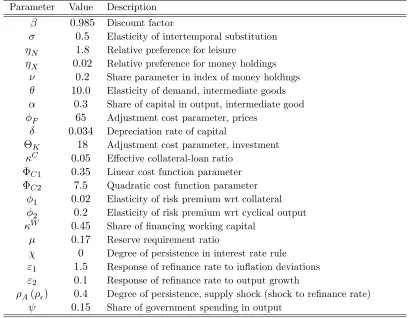
Table 1. Calibrated Parameter Values Parameter Value Description

0:985 Discount factor

0:5 Elasticity of intertemporal substitution

N 1:8 Relative preference for leisure

X 0:02 Relative preference for money holdings

0:2 Share parameter in index of money holdings

10:0 Elasticity of demand, intermediate goods

0:3 Share of capital in output, intermediate good

F 65 Adjustment cost parameter, prices

0:034 Depreciation rate of capital

K 18 Adjustment cost parameter, investment C _{0:05 E¤ective collateral-loan ratio}

C1 0:35 Linear cost function parameter

C2 7:5 Quadratic cost function parameter 1 0:02 Elasticity of risk premium wrt collateral 2 0:2 Elasticity of risk premium wrt cyclical output

W _{0:45 Share of …nancing working capital}

0:17 Reserve requirement ratio

0 Degree of persistence in interest rate rule

"1 1:5 Response of re…nance rate to in‡ation deviations

"2 0:1 Response of re…nance rate to output growth

A( ) 0:4 Degree of persistence, supply shock (shock to re…nance rate)

0:15 Share of government spending in output

The steady-state deposit rate is set at1:05percent, which is the actual value on average for the period 2007-2011.21 _{It is important to note that the low deposit rate is due to the}

high liquidity environment, which depresses the short-term interest rate.22 _{Further, the}

data show that the prime lending rate for T&T is 10:7 percent on average during 2007-2011. This value is therefore used for the steady-state loan rate. Banks in T&T earn no interest on primary reserve requirements. However, the Central Bank pays interest on secondary reserve requirements.23 These secondary reserve balances are remunerated at

350 basis points below the policy interest rate. The interest rate paid on reserves is set

2 1_{This represents the deposit rate announced by commercial banks for ordinary savings.}

2 2_{Similarly, inspection of the data shows that the rise in excess reserves in the United States and Euro}

Area in recent years was associated with a sharp fall in the short-term interest rate.

2 3_{E¤ective October 2006, commercial banks were required to hold, on a temporary basis, 2percent of}

at a low value of0:25 percent, which satis…es the condition that the interest rate on total reserves is less than the re…nance rate. The ratio of excess reserves to total reserves in the steady state is 20:9 percent, which is close to the value observed in the recent data for T&T. Further, in the steady state, the proportion of deposits held as total reserves is 21:5 percent. The steady-state value of the repayment probability is 97 percent; this implies the default probability is around3percent. The steady-state ratio of consumption to output is68:1 percent, which is close to the value of 66:8 percent for the period 2007-2011. For the same period, the cash plus deposit to output ratio is 49:3 percent; hence the steady-state value is set at 45:2 percent, which is a close approximation of the actual value. Also, in the steady state the ratio of investment to output is set at 16:8 percent, while the collateral-to-loan ratio is 1:47.

6

Policy Analysis

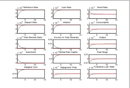
This section uses impulse response functions to study the dynamic e¤ects of four shocks to the model. All the …gures show the percent deviation of the variables from their steady-state values, with the exception of the total reserve ratio, in‡ation and the interest rate variables which are expressed in percentage points. The …rst case examines the impact of a negative supply shock. We then analyse the transmission of monetary policy following an increase in the central bank’s re…nance rate. The next experiment investigates the impact of a shock to reserve requirements. Following this, we examine the response of the model to a liquidity shock, taking the form of an increase in bank deposits. Finally, simultaneous shocks are administered to deposits and the required reserve ratio.

6.1 Negative Supply Shock

central bank’s real bond holdings, which determine the total monetary assets, are …xed, the bond rate adjusts to clear the money market. Therefore, to reduce the demand for cash, the bond rate increases, which, through intertemporal substitution, leads to a fall in the level of current consumption. Overall, the higher rate of return on deposits and bonds increases households’ demand for these …nancial assets, and lowers their consumption.

A key point to note is that based on the calibration, the cost channel exists ( W >0). Therefore, owing to the fact that marginal costs depend directly on the policy interest rate, an increase in this rate tends to further raise …rms’ marginal costs as it increases the labour costs of production. Furthermore, the increase in the re…nance rate also translates to an immediate rise in the loan rate, which lowers the demand for investment and the level of physical capital over time. The collateral-to-loan ratio increases on impact as loans for investment fall by more than the value of collateral. Because the collateral e¤ect is dominated by the cyclical output e¤ect, the repayment probability falls, causing the loan rate to increase further, which in turn exerts an upward pressure on the rental rate of capital. Based on the calibration, the higher rental rate of capital o¤sets the fall in the level of physical capital, the rise in both labour supply and the re…nance rate, causing real wages to increase upon the impact of the shock.24 The rise in real wages, in turn, creates further upward pressure on …rms’ marginal costs.

In this model, excess reserves are positively related to their rate of return, but depend negatively on the re…nance rate. Therefore, because the interest rate paid on reserves is …xed by the central bank, an increase in the marginal cost of borrowing from the central bank lowers the level of excess reserves. As the re…nance rate and the other interest rates in the banking sector increase, the costs of holding excess reserves are higher. Put di¤erently, there is a higher opportunity cost of holding excess reserves when the marginal cost of borrowing from the central bank increases. Thus, provided that the interest rate on reserves remains unchanged, the rise in other short-term interest rates indicates that banks can earn a higher return from investing in other assets, so they reduce demand for excess reserves. Given that the excess reserve ratio decreases, and that the required reserve ratio remains constant, the total reserve ratio also falls.

2 4_{The value of capital, labour supply, the re…nance rate and the rental rate of capital were calculated.}

Figure 2. Negative Supply Shock (Deviations from Steady State)

5 10 15

0 0.5 1

Refinance Rate

5 10 15

0 0.5 1

Loan Rate

5 10 15

0 0.5 1

Bond Rate

5 10 15

0 0.5 1

Deposit Rate

5 10 15

0 0.5 1

Inflation

5 10 15

-0.4 -0.2 0

Consumption

5 10 15

-0.4 -0.2 0

Total Reserve Ratio

5 10 15

-2 -1 0

Excess to Total Reserves

5 10 15

-1 -0.5 0

Output

5 10 15

-4 -2 0

Investment

5 10 15

0 0.05 0.1

Rental Rate Capital

5 10 15

-1 0 1

Real Wage

5 10 15

0 2 4

Marginal Cost

5 10 15

-0.1 -0.05 0

Repayment Prob.

5 10 15

-5 0 5

Collateral-Loan Ratio

6.2 Monetary Policy Shocks

6.2.1 Increase in Re…nance Rate

case, real wages fall by more than the value of physical capital, placing downward pressure on the rental rate of capital. The decline in marginal costs, which results from the drop in the rental rate of capital and real wages, creates a downward pressure on in‡ation.

Similar to the case of the negative productivity shock, the higher re…nance rate increases the opportunity cost of holding excess reserves. As a consequence, the bank demands less excess reserves. The reduction in the quantity of excess reserves leads to an immediate fall in the level of total bank reserves.

Figure 3. Increase in Re…nance Rate (Deviations from Steady State)

5 10 15

0 0.1 0.2

Refinance Rate

5 10 15

0 0.1 0.2

Loan Rate

5 10 15

0 0.05 0.1

Bond Rate

5 10 15

0 0.05 0.1

Deposit Rate

5 10 15

-1 0 1

Inflation

5 10 15

-0.4 -0.2 0

Consumption

5 10 15

-0.1 -0.05 0

Total Reserve Ratio

5 10 15

-0.4 -0.2 0

Excess to Total Reserves

5 10 15

-0.4 -0.2 0

Output

5 10 15

-2 -1 0

Investment

5 10 15

-0.2 0 0.2

Rental Rate Capital

5 10 15

-4 -2 0

Real Wage

5 10 15

-5 0 5

Marginal Cost

5 10 15

-0.1 -0.05 0

Repayment Prob.

5 10 15

-2 0 2

Collateral-Loan Ratio

6.2.2 Increase in Reserve Requirement Ratio

point increase in the minimum reserve requirement ratio, we assume that _t is stochastic and follows a …rst-order autoregressive process of the form: _t= _{t 1}exp ( _t).

The impulse response functions in Figure 4 show that an increase in reserve require-ments does indeed lead to a reduction in the excess reserve ratio. In general, because the required reserve ratio goes up and the excess reserve ratio falls, the net e¤ect on the total reserve ratio is a priori ambiguous; given our calibration, the net e¤ect is positive, as shown in the simulations. Because the deposit rate is set as a mark-down on the total reserve ratio, a rise in total reserves leads to a fall in the interest rate on deposits. Con-sequently, household deposits fall, while borrowing from the central bank and the money supply increase. Equilibrium in the money market requires an increase in the demand for cash, which is brought about through a reduction in the bond rate, which in turn leads to a higher level of current consumption and output. The policy rate increases in response to the rise in output. Furthermore, an increase in the marginal cost of borrowing from the central bank leads to a rise in the loan rate, which results in a higher rental rate of capital, a decline in investment and a lower capital stock over time. Primarily owing to the higher rental rate of capital, real wages increase. As observed previously, a higher lending rate leads to a reduction in investment loans, and a rise in the collateral-to-loan ratio. The higher output, along with the increase in the collateral-to-loan ratio, cause the repayment probability to rise. Nevertheless, the increase in the re…nance rate dominates the response of the repayment probability, such that the loan rate rises although mitigated due to the fall in the perception of risk. Marginal costs increase because of three simultaneous e¤ects: the increase in the re…nance rate, higher real wages and the rise in the rental rate of capital. The increase in …rms’ production costs creates an upward pressure on prices, leading to an ampli…ed rise in the re…nance rate.

Therefore, similar to the results in Glocker and Towbin (2012), under an interest rate rule an increase in reserve requirements widens the spread between lending and deposit rates.25 _{Owing to the fact that the bank holds excess reserves, it is fully responsive to the}

increase in reserve requirements and therefore cuts the deposit rate to induce households to reduce their demand for deposits. The lower level of deposits, in turn, leads to a lower ratio of excess reserves, while the fall in the deposit rate stimulates consumption. The total net e¤ect of the shock on output depends on the relative changes in consumption and investment. Based on the calibration, the e¤ect of the increase in consumption dominates

2 5_{Montoro and Moreno (2011) and Tovar et al. (2012) also pointed out that an increase in required}

the fall in investment, so output rises.26 _{This implies that changes in reserve requirements}

are procyclical, with respect to economic activity.27

Figure 4. Increase in Reserve Requirement Ratio (Deviations from Steady State)

5 10 15

0 2 4x 10

-3 _{Refinance Rate}

5 10 15

0 1 2x 10

-3 _{Loan Rate}

5 10 15

-1 0 1x 10

-3 _{Bond Rate}

5 10 15

-1 0 1x 10

-3_{Deposit Rate}

5 10 15

0 1 2x 10

-3 _Inflation

5 10 15

-1 0 1x 10

-3 _Consumption

5 10 15

0 0.5 1

Total Reserve Ratio

5 10 15

-0.04 -0.02 0

Excess to Total Reserves

5 10 15

-1 0 1x 10

-3 _Output

5 10 15

-4 -2

0x 10

-5 _Investment

5 10 15

0 2 4x 10

-4_{Rental Rate Capital}

5 10 15

-5 0 5x 10

-3 _{Real Wage}

5 10 15

0 0.005 0.01

Marginal Cost

5 10 15

-2 0 2x 10

-4 _{Repayment Prob.}

5 10 15

-5 0 5x 10

-5_{Collateral-Loan Ratio}

2 6_{In the case of a decrease in reserve requirements, the deposit rate rises and the loan rate falls. The}

fall in the loan rate increases investment, while the rise in the deposit rate reduces consumption. Usually, the overall e¤ect brings about a fall in output because the drop in consumption dominates the increase in investment. The …ndings from a study by Areosa and Coelho (2013) showed that a decrease in reserve requirements caused output to increase. It must however be noted that in their study, the condition speci…ed for the loan rate (which was not derived optimally) ensured that a lower reserve requirement ratio generated an overall countercyclical e¤ect.

2 7_{See Horrigan (1988) and Baltensperger (1982) for further discussions on the impact of changes in reserve}

6.3 Liquidity Shock: Increase in Bank Deposits

Figure 5. Increase in Bank Deposits (Deviations from Steady State)

5 10 15

-4 -2

0x 10

-3_{Refinance Rate}

5 10 15

-4 -2

0x 10

-3 _{Loan Rate}

5 10 15

-2 0 2x 10

-3 _{Bond Rate}

5 10 15

-4 -2

0x 10

-3 _{Deposit Rate}

5 10 15

-4 -2

0x 10

-3 _Inflation

5 10 15

-2 0 2x 10

-3 _Consumption

5 10 15

0 2 4x 10

-3_{Total Reserve Ratio}

5 10 15

0 0.01 0.02

Excess to Total Reserves

5 10 15

-2 0 2x 10

-3 _Output

5 10 15

0 1 2x 10

-4 _Investment

5 10 15

-1 -0.5

0x 10

-3_{Rental Rate Capital}

5 10 15

-0.01 0 0.01

Real Wage

5 10 15

-0.02 -0.01 0

Marginal Cost

5 10 15

-5 0 5x 10

-4 _{Repayment Prob.}

5 10 15

-2 0 2x 10

-4_{Collateral-Loan Ratio}

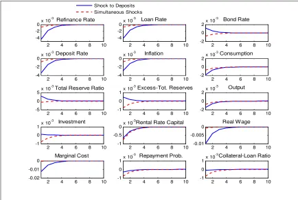
6.4 Simultaneous Shocks to Deposits and Reserve Requirements

also be noted that under the combined shock, there is lower volatility for the interest rate variables. Notably, ‡uctuations in in‡ation and output are also reduced.

Figure 6. Increase in Bank Deposits and Simultaneous Shocks to Deposits and Reserve Requirements (Deviations from Steady State)

2 4 6 8 10

-4 -2

0x 10

-3 _{Refinance Rate}

2 4 6 8 10

-4 -2

0x 10

-3 _{Loan Rate}

2 4 6 8 10

-2 0 2x 10

-3 _{Bond Rate}

2 4 6 8 10

-4 -2

0x 10

-3_{Deposit Rate}

2 4 6 8 10

-4 -2

0x 10

-3 _Inflation

2 4 6 8 10

-2 0 2x 10

-3_Consumption

2 4 6 8 10

-5 0 5x 10

-3

Total Reserve Ratio

2 4 6 8 10

-1 0 1x 10

-3_{Excess-Tot. Reserves}

2 4 6 8 10

-2 0 2x 10

-3 _Output

2 4 6 8 10

-1 0 1x 10

-3 _Investment

2 4 6 8 10

-1 -0.5

0x 10 -3

Rental Rate Capital

2 4 6 8 10

-0.01 -0.005 0

Real Wage

2 4 6 8 10

-0.02 -0.01 0

Marginal Cost

2 4 6 8 10

-1 0 1x 10

-3 _{Repayment Prob.}

2 4 6 8 10

-1 0 1x 10

-3_{Collateral-Loan Ratio} Shock to Deposits

Simultaneous Shocks

7

Policy Rules for Managing Excess Reserves

This section examines the macroeconomic e¤ects of a liquidity shock when two alternative policy rules are used - an augmented Taylor rule and a countercyclical rule for the required reserve ratio.

7.1 An Augmented Taylor Rule

the main variables of the model, under a shock to deposits. The augmented interest rate rule takes the following form,

^{R_t = ^{R_{t 1}+ (1 )["1(^t) +"2( ^Yt) +"3(ER\_T Rt)] + t; (53)

where ER\_T R_t denotes the ratio of excess reserves to total reserves in log-linear form. Primus (2012) estimated an augmented Taylor rule for Trinidad and Tobago which in-cluded a measure of excess reserves. The results from her study showed the relative weight corresponding to deviations in excess reserves from steady-state,"3, is 0:03. The negative

coe¢cient indicates that in response to an increase in excess reserves, the central bank low-ers the policy rate to reduce incentive for banks to hold excess liquidity. Intuitively, if the penalty rate for not meeting the reserve requirement is low, commercial banks would tend to reduce their holdings of excess reserves. By contrast, if the penalty rate is high, banks would voluntarily hold excess reverses as a measure of precaution to avoid any shortfall in liquidity. A reduction in the policy rate is also expected to lower the deposit rate, which in turn discourages household deposits.

The estimated value of 0:03is quite low and had only a marginal e¤ect on the policy rule and the model by extension. As a result of this, we consider alternative values of

0:05 and 0:2 for"3. To assess the impact of an augmented policy rule on volatility, we

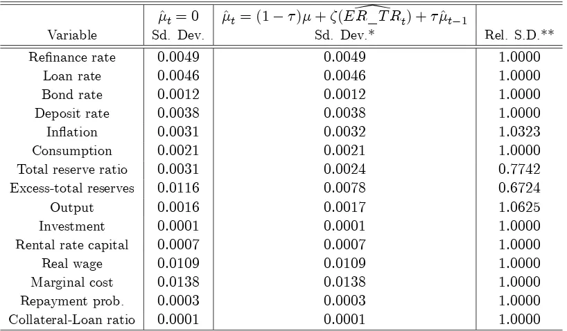
compare the asymptotic standard deviations and the relative standard deviations of the main variables in the model under a liquidity shock with the augmented Taylor rule and the standard Taylor rule (see Table 2). Figure 7 compares the simulations of a shock to deposits under both rules when "3 is set at 0:2. The results from Figure 7 and Table 2 indicate

Figure 7. Increase in Bank Deposits under Standard Taylor Rule and Augmented Taylor Rule (Deviations from Steady State)

2 4 6 8 10

-4 -2

0x 10

-3_{Refinance Rate}

2 4 6 8 10

-4 -2

0x 10

-3 _{Loan Rate}

2 4 6 8 10

-2 0 2x 10

-3 _{Bond Rate}

2 4 6 8 10

-4 -2

0x 10

-3_{Deposit Rate}

2 4 6 8 10

-4 -2

0x 10

-3 _Inflation

2 4 6 8 10

-2 0 2x 10

-3_Consumption

2 4 6 8 10

0 2 4x 10

-3_{Total Reserve Ratio}

2 4 6 8 10

0 0.005 0.01

Excess to Total Reserves

2 4 6 8 10

-2 0 2x 10

-3 _Output

2 4 6 8 10

0 2 4x 10

-3 _Investment

2 4 6 8 10

-1 -0.5

0x 10

-3

Rental Rate Capital

2 4 6 8 10

-0.01 0 0.01

Real Wage

2 4 6 8 10

-0.02 -0.01

0 Marginal Cost

2 4 6 8 10

-5 0 5x 10

-4

Repayment Prob.

2 4 6 8 10

-5 0 5x 10

-3

Collateral-Loan Ratio

Std. Taylor Rule Aug. Taylor Rule

Table 2. Standard Deviations under Standard Taylor Rule and Augmented Taylor Rule with Increase in Bank Deposits

"3= 0 "3= 0:03 "3= 0:05 "3= 0:2

Variable Sd. Dev. Sd. Dev.* Rel. S.D.** Sd. Dev. Rel. S.D. Sd. Dev. Rel. S.D. Re…nance rate 0:0049 0:0049 1:0000 0:0049 1:0000 0:0051 1:0408

Loan rate 0:0046 0:0046 1:0000 0:0047 1:0217 0:0050 1:0870

Bond rate 0:0012 0:0012 1:0000 0:0012 1:0000 0:0011 0:9167

Deposit rate 0:0038 0:0038 1:0000 0:0039 1:0263 0:0040 1:0526

In‡ation 0:0031 0:0029 0:9355 0:0028 0:9032 0:0018 0:5806

Consumption 0:0021 0:0020 0:9524 0:0019 0:9048 0:0014 0:6667

Total reserve ratio 0:0031 0:0031 1:0000 0:0031 1:0000 0:0032 1:0323

Excess-total reserves 0:0116 0:0117 1:0086 0:0118 1:0172 0:0122 1:0517

Output 0:0016 0:0015 0:9375 0:0014 0:8750 0:0006 0:3750

Investment 0:0001 0:0005 5:0000 0:0008 8:0000 0:0030 30:0000

Rental rate capital 0:0007 0:0007 1:0000 0:0006 0:8571 0:0004 0:5714

Real wage 0:0109 0:0100 0:9174 0:0095 0:8716 0:0051 0:4679

Marginal cost 0:0138 0:0129 0:9348 0:0123 0:8913 0:0077 0:5580

Repayment prob. 0:0003 0:0003 1:0000 0:0003 1:0000 0:0002 0:6667

Collateral-Loan ratio 0:0001 0:0005 5:0000 0:0008 8:0000 0:0030 30:0000

7.2 A Countercyclical Reserve Requirement Rule

In the second case we investigate the macroeconomic e¤ects of a policy rule in which the required reserve ratio is determined by its previous value, a fraction of its steady-state value, and deviations in excess reserves. Therefore, in this approach, the required reserve ratio is endogenous and serves a countercyclical role for managing changes in excess reserves. The central bank is assumed to set the reserve requirement rule according to the following,

^_t= (1 ) + (ER\_T R_t) + ^_{t 1}; (54) where denotes the degree of persistence in the policy rule and , which measures devia-tions in the ratio of excess reserves to total reserves from its steady-state, is an indicator of cyclical conditions. There is little information on the values for and . Our numeric experiments suggest a value of 0:12 for , and 0:85 for . Thus, there is a relatively low degree of persistence in changes of the required reserve ratio. Also, the positive value for means that the central bank increases required reserves when there is a rise in excess bank liquidity.