Finding and proving the exact ground state of a generalized Ising model by convex optimization
and MAX-SAT
Wenxuan Huang,1Daniil A. Kitchaev,1Stephen T. Dacek,1Ziqin Rong,1Alexander Urban,3Shan Cao,1 Chuan Luo,2and Gerbrand Ceder1,3,4,*
1Department of Material Science and Engineering, Massachusetts Institute of Technology, Massachusetts 02139, USA 2Institute of Computing Technology, Chinese Academy of Sciences, Beijing 100190, China
3Department of Materials Science and Engineering, University of California, Berkeley, Berkeley, California 94720, USA 4Materials Science Division, Lawrence Berkeley National Laboratory, Berkeley, California 94720, USA
(Received 28 April 2015; revised manuscript received 30 May 2016; published 21 October 2016) Lattice models, also known as generalized Ising models or cluster expansions, are widely used in many areas of science and are routinely applied to the study of alloy thermodynamics, solid-solid phase transitions, magnetic and thermal properties of solids, fluid mechanics, and others. However, the problem of finding and proving the global ground state of a lattice model, which is essential for all of the aforementioned applications, has remained unresolved for relatively complex practical systems, with only a limited number of results for highly simplified systems known. In this paper, we present a practical and general algorithm that provides a provable periodically constrained ground state of a complex lattice model up to a given unit cell size and in many cases is able to prove global optimality over all other choices of unit cell. We transform the infinite-discrete-optimization problem into a pair of combinatorial optimization (MAX-SAT) and nonsmooth convex optimization (MAX-MIN) problems, which provide upper and lower bounds on the ground state energy, respectively. By systematically converging these bounds to each other, we may find and prove the exact ground state of realistic Hamiltonians whose exact solutions are difficult, if not impossible, to obtain via traditional methods. Considering that currently such practical Hamiltonians are solved using simulated annealing and genetic algorithms that are often unable to find the true global energy minimum and inherently cannot prove the optimality of their result, our paper opens the door to resolving longstanding uncertainties in lattice models of physical phenomena. An implementation of the algorithm is available athttps://github.com/dkitch/maxsat-ising.
DOI:10.1103/PhysRevB.94.134424
I. INTRODUCTION
Lattice models have wide applicability in science [1–10] and have been used in a wide range of applications, such as magnetism [11], alloy thermodynamics [12], fluid dynamics [13], phase transitions in oxides [14], and thermal conductivity [15]. A lattice model, also referred to as a generalized Ising model [16] or cluster expansion [12], is the discrete representation of material properties, e.g., formation energies, in terms of lattice sites and site interactions. In first-principles thermodynamics, lattice models take on a particularly important role as they appear naturally through a coarse graining of the partition function [17] of systems with substitutional degrees of freedom. As such, they are invaluable tools for predicting the structure and phase diagrams of crystalline solids based on a limited set of ab initio
calculations [18–22]. In particular, the ground states of a lattice model determine the 0 K phase diagram of the system. However, the procedure to find and prove the exact ground state of a lattice model, defined on an arbitrary lattice with any interaction range and number of species, remains an unsolved problem, with only a limited number of special-case
Published by the American Physical Society under the terms of the
Creative Commons Attribution 3.0 License. Further distribution of this work must maintain attribution to the author(s) and the published article’s title, journal citation, and DOI.
solutions known in the literature [23–29].In general systems, an approximation of the ground state is typically obtained from Monte Carlo (MC) simulations, which by their stochastic nature can prove neither convergence nor optimality. Thus, in light of the wide applicability of the generalized Ising model, an efficient approach to finding and proving its true ground states would not only resolve longstanding uncertainties in the field and give significant insight into the behavior of lattice models, but would also facilitate their use inab initio
thermodynamics.
found and proven, we argue that our algorithm significantly improves on the state-of-the-art in computational efficiency and does not sacrifice any guarantees of optimality with respect to established methodology.
II. NOTATION AND BACKGROUND
A lattice model is a set of fixed sites on which objects (spins, atoms of different types, vacancies, etc.) are to be distributed. Its Hamiltonian consists of coupling terms between pairs, triplets, and other groups of sites, which we refer to as “clusters”. A formal definition of effective cluster interactions can be found in Ref. [12]. Before discussing the algorithmic details of our method, it is essential to establish a precise mathematical definition of a general lattice model Hamiltonian and the task of determining its ground states. The ground state problem can formally be stated as follows: Given a set of effective cluster interactions (ECIs)J ∈RC, whereCis the set of interacting clusters andRis the set of real numbers, what is the configurations:D→ {0,1}, whereDis the domain of configuration space, such that the global Hamiltonian H is minimized:
min
s H =mins Nlim→∞ 1 (2N+1)3
×
(i,j,k)∈{−N,...,N}3
α∈C
Jα
(x,y,z,p,t)∈α
Si+x,j+y,k+z,p,t
(1)
In the Hamiltonian given by Eq. (1), each α∈C is an individual interacting cluster of sites. In turn, each site within α is defined by a tuple (x,y,z,p,t), wherein (x,y,z) is the index of the primitive cell containing the interacting site,p denotes the index of the subsite to distinguish between multiple sublattices in that cell, and t is the species occupying the site. To discretize the interactions, we introduce the “spin” variablessx,y,z,p,t, where sx,y,z,p,t =1 indicates that thepth subsite of the (x,y,z) primitive cell is occupied by speciest, and otherwise,sx,y,z,p,t =0. The energy can be represented in terms of spin products, where each clusterαis associated with an ECIJαdenoting the energy associated with this particular cluster. To obtain the energy of the entire system, each cluster needs to be translated over all possible periodic images of the primitive cell, i.e., we have to consider all possible translations of the interacting cluster α, defined as a set of (x,y,z,p,t), by (i,j,k) primitive cell translations, yielding the spin product(x,y,z,p,t)∈αsi+x,j+y,k+z,p,t. Finally, the prefactor
1
(2N+1)3 normalizes the energy to one lattice primitive cell, and the limit ofNapproaching infinity emphasizes our objective of minimizing the average energy over the entire infinitely large lattice. One remaining detail is that the Hamiltonian given in Eq. (1) is constrained such that each site in the lattice must be occupied. For the sake of simplicity, lattice vacancies are included as explicit species in the Hamiltonian, so that all spin variables associated with the same site sum up to one:
t∈c(p)
[image:2.608.326.546.70.269.2]sx,y,z,p,t =1∀(x,y,z,p)∈F. (2)
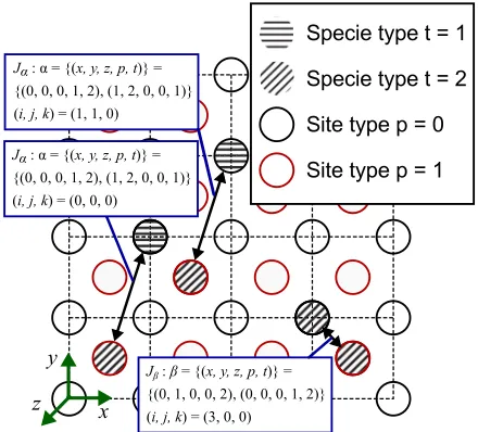
FIG. 1. Illustration of a lattice Hamiltonian and examples of cluster interactions. The primitive unit of the lattice is indicated by a thin dashed line, and sites are represented by circles. Two different site types are distinguished by black and red borders, respectively. The nonvacancy species that can occupy the sites are indicated by two different hatchings.
In Eq. (2),Fis the set of all sites in the form of (x,y,z,p), andc(p) denotes the set of species that can occupy subsitep. The domain of configuration spaceDcan be formally defined as the set of all (x,y,z,p,t), witht ∈c(p).
To further illustrate the notation introduced above, Fig.1 depicts an example of a two-dimensional (2D) lattice Hamil-tonian for a square lattice with two subsites in each lattice primitive cell, i.e.,p∈ {0,1}. Each subsite may be occupied by three types of species, so that t ∈ {0,1,2}, where t =0 shall be the reference (for example, vacancy) species. Hence, the energy of the system relative to the reference can be encoded into t ∈ {1,2}. Furthermore, the Hamiltonian shall be defined by only two different pairwise interaction types with the associated clustersα= {(0,0,0,1,2),(1,2,0,0,1)}and β= {(0,1,0,0,2),(0,0,0,1,2)}, and thus, the set of all clusters isC= {α,β}. The first three of the five indices in parentheses indicate the initial unit cell position, the fourth index corre-sponds to the position in the unit cell (subsite index), and the last index gives the species. The third component of the cell index (x,y,z) was retained for generality but set to 0 for this 2D example. The example configuration shown in Fig.1depicts three specific interactions: The interaction represented on the bottom left in the figure is of typeαwith (i,j,k)=(0,0,0), corresponding to the spin productJαs0,0,0,1,2·s1,2,0,0,1. The
interaction in the center of the figure also belongs to type α, but with (i,j,k)=(1,1,0), corresponding to the spin product Jαs0+1,0+1,0,1,2·s1+1,2+1,0,0,1=Jαs1,1,0,1,2·s2,3,0,0,1.
Lastly, the interaction on the right represents an interacting β cluster, with (i,j,k)=(3,0,0), yielding a spin product of Jβs0+3,1,0,0,2s0+3,0,0,1,2=Jβs3,1,0,0,2s3,0,0,1,2.
it is inherently an optimization over a finite set of sites, whereas the true objective function is defined over an infinite number of sites. Second, the result obtained from a MC calculation is simply a particular low-energy configuration, a local minimum of energy, with no guarantee that it is the true ground state. This limitation becomes especially problematic when the size of the ground state structure increases, since the large number of degrees of freedom quickly renders it infeasible to sample the low-energy configurations in the cell. Hence, due to its stochastic nature and dependence on a particular lattice supercell, simulated annealing can only identify possible ground state candidates, but it can hardly guarantee that the global ground state has been found.
An alternative approach that provides a provable ground state is the configurational polytope method [32,33] com-bined with vertex enumeration [34]. This method provides a beautiful reformulation of the ground state problem as linear programming (LP). Unfortunately, this approach has not been applied to finding the ground states of complex realistic Hamiltonians due to its computational inefficiency and the fact that the method yields a polytope with an large number of “inconstructible” vertices, i.e solutions that do not correspond to realizable lattice configurations, and there is no general, tractable algorithm to extract the true constructible polytope [35,36]. Recently, the “basic ray” method has been proposed and used to obtain the ground states of several small systems [23–25]. However, a universal algorithm based on this method is not known [24], and the number of systems solved by this approach is limited.
In the following, we present a computationally efficient algorithm that is able to provide a provable periodically constrained ground state up to a set unit cell size and, in many cases, prove that this ground state is the exact ground state of the generalized Ising Hamiltonian over infinite space. We derive the algorithm, demonstrate its applicability to arbitrary lattices and general multicomponent systems, and demonstrate its computational performance for practically relevant systems. Finally, we compare our algorithm to the state-of-the-art polytope method and discuss the relationship between the two methods, the guarantees of optimality they are able to provide, and their relative computational efficiency.
An implementation of this method, along with several examples, is available in Ref. [37].
III. METHOD FORMULATION
Our general scheme for finding an exact ground state of an Ising model is to calculate and converge upper and lower bounds on the energy. We note that the energy of any periodic configuration is an upper bound on the ground state energy [38]. Thus, by enumerating periodicities and finding the exact ground state for each, we can successively tighten the upper bound on the true ground state energy. If an exact periodic ground state structure exists, we are guaranteed to obtain the tightest upper bound possible once we reach the true periodicity by enumeration. However, there is no way of knowing when this condition has been reached, i.e., when the enumeration should stop. We therefore require an additional procedure to construct successfully tighter, rigorous lower bounds on the ground state energy, so that periodicity
enumeration can be stopped when the upper and lower bounds match, indicating that the exact ground state has been found. Our approach for the construction of the lower bound is less intuitive and involves the optimization over a nonperiodic domain. We discuss both upper- and lower-bound procedures separately.
Note that cluster expansions are often applied in both canonical and grand canonical contexts, i.e., investigating the ground states that arise at both fixed composition and fixed chemical potential [39,40]. Our derivation focuses on the grand canonical case, where the chemical potential of each species is fixed by the “single-point” interaction terms. However, the grand canonical solution obtained this way can be readily used to obtain the canonical ground states using a convex hull approach [41]. By construction, it removes compositions that do not have a stable ground state. In thermodynamic language, we minimize the Legendre transform of the energy (grand potential) with respect to composition, rather than the energy itself, as is the common procedure to find ground states as a function of composition [39].
A. Enumerating periodicity
We begin our optimization of the upper bound on the energy by enumerating all distinct periodicities up to a chosen maximal unit cell size, which can be iteratively increased until convergence of the upper and lower bounds has been obtained. Note that all distinct periodic orderings on a lattice can be represented by an all-integer supercell matrix in Hermite normal form [42], whose determinant represents the size of the periodic super cell. Thus, we can systematically enumer-ate all periodicities by generating supercells of the lattice primitive cell from all integer Hermite normal form matrices up to a given determinant. We then proceed to solve the fixed-periodicity ground state problem within each generated supercell, achieving successively tighter upper bounds on the infinite-lattice ground state energy.
B. Obtaining the ground state at a fixed periodicity The first element of our solution to the ground state problem is to efficiently find the ground state given a fixed periodicity of the solution. While this problem is typically solved by Metropolis MC simulated annealing in a prescribed simulation cell, this approach cannot prove that the periodic solution found is in fact optimal, even for a given periodicity.
of optimization problems for which highly efficient solvers exist [46,47].
Using the notation introduced in the previous section, we note that calculating the periodic ground state is equivalent to solving the finite optimization problem:
min s
α∈C˜
Jα
(x,y,z,p,t)∈α
sx,y,z,p,t (3)
subject to:
t∈c(p)
sx,y,z,p,t =1∀(x,y,z,p)∈Ffinite (4)
where
sx,y,z,p,t is, as s in Eq. (2), the indicator variable of speciest on site (x,y,z,p), with the difference thats
is now defined on a smaller domain determined by the periodicity;C˜
is the set of all interacting clusters within the fixed periodic
system; andFfinite is the set of sites within the fixed periodic
unit cell. Such an optimization over discrete{0,1}variables can be equivalently posed as a logic problem by converting the minimization problem into the negative of a maximization problem and replacing the discrete variables by Boolean equivalents. Following this insight, the minimization of the finite Hamiltonian can be expressed in the form of a PBO problem, allowing us to solve this optimization as a weighted partial maximum satisfiability (MAX-SAT) [46,47] problem. The essence of MAX-SAT is to model the discrete optimization problem by maximizing the number of logical clauses that can be satisfied in a Boolean formula of conjunctive normal form, weighted by a set of arbitrary coefficients.
To illustrate this approach, we consider the example of a binary one-dimensional (1D) system with a positive point term J0and a negative nearest-neighbor interactionJN N, on a 2-site
unit cell. For this system, the transformation is:
E= min s
0,s1
(J0s0+J0s1+JN Ns0s1)
= −max[J0(1−s0)−J0+J0(1−s1)−J0−JN N(s0s1)] = −max{J0(¬s0)−J0+J0(¬s1)−J0+(−JN N)[(1− ¬s0)s1]}
= −max[J0(¬s0)−J0+J0(¬s1)−J0+(−JN N)s1+(−JN N)(1− ¬s0s1)−(−JN N)]
=(2J0−JN N)−MAXSAT[J0(¬s0)∧J0(¬s1)∧(−JN N)(s1)∧(−JN N)(s0∨ ¬s1)], (5)
where the indicator variable
si is now also a Boolean variable in the MAX-SAT setting, and the ∧, ∨ and ¬ operators correspond to logical “and”, “or”, and “not”, respectively. Note that, although in a MAX-SAT problem the coefficient of each clause needs to be positive, it is still possible to transform an arbitrary set of cluster interactionsJiinto a proper MAX-SAT input, as in the example above.
The advantage of formulating the ground state problem in this form is that MAX-SAT is one of the most ac-tively researched non-deterministic polynomial-time (NP)-hard problems [48], allowing us to leverage the extensive literature written on the topic [49–52]. Note that any complete MAX-SAT solver encodes a proof of optimality [50] and includes a published proof of algorithm correctness (that it is guaranteed to find the optimal solution) [46] and efficiency [51,52]. Furthermore, the algorithms are run through an annual MAX-SAT competition [49], which tests their correctness, robustness, and efficiency. Under such stringent criteria, by converting our problem into MAX-SAT, we can safely guarantee provability, as well as further investigate the advanced proof schemes and fast algorithms developed over the last 20 years of MAX-SAT research [46,47,50]. The particular MAX-SAT solver we chose, based on the results of the MAX-SAT 2014 competition benchmarking and our own testing, is CCLS_to_akmaxsat [47,53].
Another notable advantage of MAX-SAT over MC for obtaining a solution of the ground state problem is that state-of–the-art MAX-SAT solvers generally include sophis-ticated methods to escape from local minima [51,52] to
arrive at the global minimum faster and more robustly than MC.
To verify the efficiency, robustness, and accuracy of the MAX-SAT solver compared to conventional MC, we performed a series of tests of both algorithms. We constructed a set of random 1D and 2D pair-interaction Hamiltonians with interactions up to the 28th nearest neighbor in 1D and up to the 10th nearest neighbor in 2D. We then attempted to find the ground state of each system within unit cells containing up to 50 sites by MAX-SAT and MC. Finally, we considered only those Hamiltonians which could be classified as “difficult”, which we define as having a ground state unit cell with more than 4 sites in 1D, or more than 12 sites in 2D. Among these “difficult” Hamiltonians, while our MAX-SAT approach consistently provides a provable ground state under the imposed periodicity constraints, we find that MC is unable to find the ground state energy comparable to the MAX-SAT result in 10% of cases. Thus, the MAX-SAT approach by itself is an attractive method to obtain provably optimal, periodically constrained ground states up to some maximum unit cell size, separate from the problem of proving the optimality of the solution over infinite space.
C. Lower-bound calculation
previous section. We must reiterate that the periodicity-constrained upper-bound solutions described previously are already guaranteed to be optimal within the periodicity constraints provided, such that the lower-bound calculation only serves as a proof that the solution obtained by periodicity enumeration is optimal over all other possible periodicities.
To start, we prove that minimization of the Hamiltonian on a finite group of sites, without any periodic constraints, provides a lower bound for the ground state energy. To see why this statement is true, consider the bounds on the Hamiltonian:
H(s)= lim N→∞
1 (2N+1)3
×
(i,j,k)∈
{−N,...,N}3
α∈C
Jα
(x,y,z,p,t)∈α
si+x,j+y,k+z,p,t (6a)
≡ lim N→∞
1 (2N+1)3
(i,j,k)∈ {−N,...,N}3
Ei,j,k,s min i,j,kEi,j,k,s
min
s0∈{0,1}BEs0 (6b)
where Ei,j,k,s is defined as
α∈CJα
(x,y,z,p,t)∈αsi+x,j+y,k+z,p,t and represents the energy of a block configuration in the lattice at location (i,j,k) for a specific s. Also, Bis the block cluster containing the relevant (x,y,z,p,t); formallyB=Uα∈Cα. Thens0∈ {0,1}B is naturally defined as a block configuration and Es0 as the
energy corresponding to block configurations0.
The first part of Eq. (6b) is a restatement of the total average energy as an average over (i,j,k) of block configuration energiesEi,j,k,s. As the left-hand-side of Eq. (6b) is an average over (i,j,k) ofEi,j,k,s, it must be greater than or equal to the minimum over (i,j,k) ofEi,j,k,s, the second part of Eq. (6b). Hence, a minimization ofEi,j,k,sover configuration space (the right-hand-side), provides a lower bound:
H(s) min s0∈{0,1}B
Es0. (7)
As an example, consider a simple binary 1D lattice system with interactions up to the next nearest neighbor (NNN). The energy of this system is bounded from below by the energy of the lowest energy block configuration:
H = lim N→∞
1 (2N+1)
(i)∈{−N,...,N}3
(J0si+J1sisi+1+J2sisi+2)
min
s0,s1,s2
(J0s0+J1s0s1+J2s0s2). (8)
Thus, minimization over the block configurations (s0,s1,s2) produces a valid lower bound, mins0,s1,s2 (J0s0+J1s0s1+J2s0s2), to the exact ground state energy.
Expressing the Hamiltonian in the above form assigns all weights of the point term interaction J0 to the 0th site of the block cluster, corresponding to a J0s0 term in the
energy. We could have just as well redistributed the point term energy over all sites in the block cluster, transforming J0s0 into 13(J0s0+J0s1+J0s2), and similarly J1s0s2 into
1
2J1(s0s2+s1s3):
H = lim N→∞
1 (2N+1)
(i)∈{−N,...,N}3
1
3(J0si+J0si+1+J0si+2)
+1
2J1(sisi+1+si+1si+2)+J2sisi+2
min
s0,s1,s2
1
3(J0s0+J0s1+J0s2)
+1
2J1(s0s2+s1s3)+J2s0s2
. (9)
In the case of the exact infinite system Hamiltonian, this transformation simply corresponds to interchanging the order of the summation and thus imparts no difference to the total energy. However, in the case of the lower bound, we have obtained a new bounding condition, which is a key insight we will use to systematically obtain the tightest possible lower bound on the ground state energy.
D. Tightening the lower bound using translationally equivalent ECIs
Generally, the direct minimization ofEs0as described in the previous section gives a very loose lower bound. In principle, a tighter lower bound could be generated systematically by enlarging the block size |B| used for finite minimization without periodicity constraints, thereby guaranteeing conver-gence to the exact ground state, as we will show below. Furthermore, by enlarging the periodicity used for periodic minimization, the upper-bound energy is also guaranteed to converge to the exact ground state. To see why this statement is true, consider a minimization over larger and larger block clusters and the resulting block configuration s0. We could then translate and duplicate the configurations0 to arrive at a periodic configurationsover the entire lattice. The energy ofs,Es, will differ from the configuration energy ofs0,Es0,
only at the block boundaries, and the difference will diminish as blocks become larger and larger. This diminishing property results from the fact that the bulk energy scales asr|D|and the boundary energy scales asr|D|−1, whereDis the dimension of
the physical system andris the size of the cubic block cluster. Here,Es0−Es therefore scales as
r|D|−1
r|D| =1r. Therefore, the difference betweenEs andEs0 approaches 0, while Es is an
upper bound andEs0is a lower bound of the exact ground state
energy, proving that the lower-bound energyEs0converges to the exact ground state energy. We also note that, when we perform periodic minimization with the same periodicity ass, we arrive at an upper-bound energy smaller than or equal toEs, while greater than the lower boundEs0, which proves that the
upper bound also converges to the exact ground state energy with increasing periodicity. Note that, despite the looseness of this provable bound, we observe that, in practice, our algorithm yields convergence superior to r|D|−1
r|D| = 1r, as we elaborate in the discussion section.
the block size. In the following, we present a much more efficient algorithm preserving the convergence property.
Given the original set of cluster interactions J ∈RC, a tighter lower bound can be obtained by introducing the set of equivalentJλ∈RC¯, which will be defined so as to leave the Hamiltonian of the infinite system in Eq. (1) unchanged, but will modify the Hamiltonian on a finite block. TheJλ∈RC¯are parameterized byλ∈Rn, which we define as a shift parameter. Note that, although theJλwill be defined to be equivalent to J in the sense that they leave the global Hamiltonian unchanged, finite minimization without periodicity constraints does not yield the same lower bound. Thus, we can maximize the lower-bound energy over λ to obtain the tightest lower bound on the ground state energy:
max
λ s∈{min0,1}BEλ,s. (10)
One natural way to introduce equivalentJλis by redistribut-ing an ECI over sites in the block cluster: given a fixed block clusterBto minimize over, for each clusterα∈Csuch that Jα =0, we construct a setCα such that all elementsβ ∈Cα are equivalent to clusterαwith respect to translations of the infinite lattice, and β⊆B. For each element β in Cα, we assign weightsλβ such thatβ∈Cαλβ=1, which relate the translationally equivalent ECIsJλto the original ECIs, so that for allα∈Candβ∈Cα,Jλ,β =λβJα.
Returning to the 1D example of a NNN binary system given in Eq. (8), the conversion is:
H = lim N→∞
1 (2N+1)
(i)∈{−N,...,N}3
(J0si+J1sisi+1+J2sisi+2)
= lim N→∞
1 (2N+1)
×
(i)∈{−N,...,N}3
[J0(λ1si+λ2si+1+(1−λ1−λ2)si+2)
+J1(λ3sisi+1+(1−λ3)si+1si+2)+J2sisi+2]
min
s0,s1,s2
{J0[λ1s0+λ2s1+(1−λ1−λ2)s2]
+J1[λ3s0s1+(1−λ3)s1s2]+J2s0s2}, (11)
where the last expression provides a lower bound on the ground state energy, dependent on λ. The rationale behind the λ transform is analogous to that seen in Eq. (9): We exploit the fact that we can evenly distribute cluster interactions across sites, leaving the system unchanged, but obtaining a different lower bound on the ground state energy. Note that we are not limited to partitioning point terms equally over all sites, i.e., we could assign a contribution of the point term energy to site 0 with weightλ1, to site 1 with λ2, and
to site 2 with 1−λ1−λ2. In this way, we can generally convertJ0s0toJ0[λ1s0+λ2s1+(1−λ1−λ2)s2], andJ1s0s2
into J1[λ3s0s1+(1−λ3)s1s2], arriving at the lower bound
expression of Eq. (11).
From this algorithm, we arrive at mins∈{0,1}BEs,λ, which is a lower bound dependent onλ. Thus,
max
λ s∈{min0,1}BEλ,s, (12)
provides the maximal lower bound in the space defined byB
andλ.
Finally, we note that Eq. (12) is a convex optimization problem. Ifsis fixed, Eλ,s is a linear function with respect toλ. Then f(λ)=mins∈{0,1}BEλ,s is the minimum of a set of linear functions evaluated atλ. Thus, f(λ) is a concave function and maxλf(λ) is a maximization over a concave function, which is equivalent to a minimization over a convex function, and thus is a convex optimization problem [54]. Due to its piecewise linear characteristic, this problem belongs to the class of nonsmooth convex optimization problems, where the objective function value is provided by MAX-SAT. In our implementation, we use the level method [55] as a subclass of the bundle method [56] to efficiently solve this optimization.
E. Further refinement of the lower bound
The introduction of equivalentJλ allows us to use finite minimization without periodicity constraints to obtain an exact lower bound on the ground state energy. Even when Eq. (12) cannot provide the exact lower bound for small|B|, by enlarging|B|and naturally introducing a higher dimensional λspace, an exact lower bound can usually be obtained. For example, in the same 1D NNN binary system, |B| can be enlarged, andλspace can be expanded as:
H = lim N→∞
1 (2N+1)
(i)∈{−N,...,N}3
(J0si+J1sisi+1+J2sisi+2)
min
s0,s1,s2,s3[J0(λ1s0+λ2s1+λ3s2+(1−λ1−λ2−λ3)s3) +J1(λ4s0s1+λ5s1s2+(1−λ4−λ5)s2s3)
+J2(λ6s0s2+(1−λ6)s1s3)]. (13)
Another alternative to introduce a refined lower bound without increasing |B| is by enlarging λ space through the introduction of new clusters. For example:
H = lim N→∞
1 (2N+1)
(i)∈{−N,...,N}3
(J0si+J1sisi+1+J2sisi+2)
min
s0,s1,s2,s3{
J0[λ1s0+λ2s1+λ3s2+(1−λ1−λ2−λ3)s3]
+J1[λ4s0s1+λ5s1s2+(1−λ4−λ5)s2s3]
+J2[λ6s0s2+(1−λ6)s1s3]+λ7s0s1s2−λ7s1s2s3}.
(14)
In cases where enlarging |B| is computationally very expensive, this second approach would be the only viable way to refine the lower bound. It remains unclear how such clusters should be introduced, given that there are, in general, an exponential number of them. However, this discussion is beyond the scope of this paper and will be addressed in future work. In this paper, exact lower bounds are obtained by enlarging|B|as demonstrated in the first example.
FIG. 2. 1D schematic illustrating (a) the energy of a global configuration, and (b) several choices of block energies, with the interaction weighted by an arbitraryλshift. The red arrows represent the point term (J0) and nearest neighbor (J1) interactions, while the blue rectangles depict tiling compatibility between adjacent blocks, ensuring that the collection of blocks sums up to the global configuration in (a).
is equal to the lower-bound value. Enlarging Dim(λ) allows higher freedom in the tiling and thus provides a more accurate lower bound. As a result, in practice, exact lower bounds are usually obtainable without much computational expense by expanding Dim(λ) naturally.
Note that, for aperiodic ground states whose representations are given in terms of tiling [57–59], this method provides a way to obtain the exact ground state, where periodicity enumeration (upper-bound calculation) is not appropriate. Thus, this method may be useful in finding aperiodic ground states on a fixed lattice.
F. Demonstration using a 1D example
To further illustrate our methodology, we present a simple 1D example to demonstrate the key ideas of our algorithm. Consider the 1D system with nearest neighbor and point term interactions (chemical potentials) shown in Fig. 2(a). The central idea of our algorithm is that the Hamiltonian can be written as an average of block energies, shown in Fig.2(b), under the constraint that the blocks whose energies we consider must sum up to the global Hamiltonian, as shown visually in Fig. 2(a), where the blocks must be able to tile to form the extended structure. Since the choice of how energy is partitioned into blocks is not unique, different ways can be used to describe the block energy, yielding the expression:
H = J0si+J1sisi+1 =
1
2J0(si+si+1)+J1sisi+1 = J0[λsi+(1−λ)si+1]+J1sisi+1, (15)
where angle brackets are used to represent averages and the terms inside the angle brackets are the so called “block energies”.
Since the global energy is the average of block energies, it must be greater than or equal to the smallest possible block energy. Thus, given interaction parameters J, the smallest possible block energy can be found through minimization over
− 1
0
1
2
λ parameter
− 3
− 2
− 1
0
1
2
3
Bloc
k
energy
(arb.units)
(0,0)
(1,1)
[image:7.608.54.290.69.227.2](0,1)
(1,0)
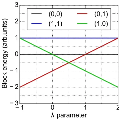
FIG. 3. Illustration of block energy in terms ofλ in the case of J0= −1 and J1=2. Each line corresponds to one block configuration whose block energy is dependent onλ.
spins in the chosen blocks, leading to a lower bound on the total energy:
H =
1
2J0(si+si+1)+J1sisi+1
min
si,si+1
1
2J0(si+si+1)+J1sisi+1
, (16)
for the case of evenly distributed point term interactions, or more generally,
H = J0[λsi+(1−λ)si+1]+J1sisi+1
min
si,si+1{
J0[λsi+(1−λ)si+1]+J1sisi+1}, (17)
for the case of aλshift. Finally, since Eq. (17) is valid for all possible choices ofλ, we can obtain a maximally tight lower bound by maximizing this expression over all possible choices ofλ:
Hmax λ smini,si+1
{J0[λsi+(1−λ)si+1]+J1sisi+1}. (18)
In this simple example, it is clear that Eq. (18) presents a convex optimization problem. By enumerating all pos-sible choices of (si,si+1) for the 1D example of Fig. 2:
(0,0),(0,1),(1,0),(1,1), Eq. (18) is
H max
λ min{0,(1−λ)J0,λJ0,J0+J1}. (19)
Each term in the curly brackets is a linear function ofλ, and therefore their minimum is concave. We illustrate this optimization in Fig.3for the case whereJ0= −1 andJ1=2.
we can guarantee that · · ·010101010· · · configuration is the global ground state even without knowing any upper bound. Furthermore, one easily verifies that· · ·010101010· · · configuration indeed has energy of−0.5. Thus, the upper and lower bounds match, proving the global optimality of this solution.
In general, for realistic systems, there are exponentially many hyperplanes with respect to the number of sites in a block cluster. One distinct advantage of our method is that we use the MAX-SAT solver to search over such exponential complexity, which as a result provides the concave function and its subgradient, which can then be used by the convex optimization solver. Naturally, due to the intrinsic complexity of the ground state problem, some NP-hard steps are unavoid-able. However, with conversion of such computationally com-plex steps into MAX-SAT, we are handling such comcom-plexity with state-of-the-art efficiency.
IV. DISCUSSION
A. Comparison to previous methods
The algorithm introduced above provides a range of important advantages over existing approaches towards ground state optimization in cluster expansions. The most common approaches to this problem in the literature are based on MC and are not adequate for proving lattice model ground states, as they only provide a loose upper bound on the energy with no way to determine convergence. Our method both improves the upper-bound calculation (by significantly reducing the prefactor in this generally NP-hard problem) and introduces an approach to derive a (typically sufficient) lower bound. The basic-rays method [23–25], a previously reported approach to the ground state problem, does not provide a lower bound on energy. Furthermore, its ground state solution to a particular set of ECIs (J) requires that basic rays are established at all vertices that define the configurational polytope facet containing J. No general approach to accomplish this has been demonstrated to work for cluster expansion systems of complexities relevant to physical systems. In contrast, our methodology is directly applicable to solving systems with a definedJ vector of relatively complex Hamiltonians, or at least provides tight bounds on the solution. To our knowledge, the only other method that can provide upper and lower bounds on lattice model ground states is the configurational polytope method [32,33] that establishes bounds on the solution by means of LP. However, as far as we know, there is no reported algorithmic system to generate the LP constraints for complex cluster expansions. Additionally, even if these constraints were known, the LP requires exponentially many variables or constraints with respect to the size of the unit cell being considered, which renders it intractable for complex Hamiltonians. Therefore, we believe that our method is unique in its ability to tackle complex Hamiltonians in a mathematically rigorous way.
B. Connection to the configurational polytope method Even though our method has been derived independently of the configurational polytope method, there exists a strong connection between our lower-bound calculation and one
form of the configurational polytope method. Namely, in relation to the most rigorous form of the configurational polytope method, which involves an exponential number of variables as it relies on strict equality constraints rather than inequalities, our approach provides a route for efficient column generation (see Ref. [60] for further details on column generation techniques in LP). This improvement expands the applicability of the method to complex, realistic Hamiltonians.
More precisely, if we start with Eq. (10) and reformulate its LP problem and its dual, Eq. (10) is equivalent to
max λ z,
s.t.: zEλ,s=
α∈C
β∈Cα
λβJα i∈β
si∀s∈ {0,1}B,
β∈Cα
λβJα=Jα∀α∈C. (20)
By reorganizing the terms, we have:
max λ z,
s.t.: z− α∈C
β∈Cα
λβJα i∈β
si 0∀s∈ {0,1}B
β∈Cα
λβJα =Jα∀α∈C. (21)
We could then apply LP to obtain its dual (groupingλβJα as one variable to allow for Jα=0). For each constraint, we construct corresponding dual variables,ρsandρα (which physically represent the “appearance frequency” of spin configurationsand clusterα, as derived later), yielding the dual problem:
min ρ
α∈C
ραJα, (22)
s.t.:
s∈{0,1}B
ρs=1, (23)
−
s∈{0,1}B
ρs
i∈β
si+ρα =0∀α∈C,β ∈Cα, (24)
ρs0 ∀s∈ {0,1}B. (25)
We arrive at one formulation of the configurational polytope method in its general form, with an exponential number of variables and constraints. We interpretρsas the probability of finding spin configurationswhen we look at some blockB, i.e., the “appearance frequency” in the configurational polytope method formulation. Therefore, the natural interpretation of Eq. (23) is that some block configuration must appear within a given block cluster, and the probability of observing all possible configurations sums to one. Similarly, Eq. (25) can be interpreted to mean that the appearance probability of each block configuration is greater than 0. Finally, Eq. (24) is the central equality that constrains the configurational polytope. It is equivalent toρα=s∈{0,1}Bρs
β, the translated interacting cluster, and i=βsi =0 oth-erwise. Therefore, ρα is the appearance probability of an interacting cluster, constrained by Eq. (24) to be translationally invariant. As a result, Eq. (22) can naturally be interpreted as a minimization of the configurational energy, with the appearance frequency of each interacting clusterραmultiplied by its interaction constantJα.
Equation (24) is the central equation that derives constraints in the configurational polytope method. For a 1D system with nearest neighbor and NNN interaction, where we takeBto be a three-site block cluster, these constraints are:
ρ[11]=ρ11∗=ρ[111]+ρ[110] =ρ[011]+ρ[111]=ρ[∗11], ρ1∗1=ρ[111]+ρ[101],
ρ[1]=ρ1∗∗=ρ[100]+ρ[101]+ρ[110]+ρ[111] =ρ∗1∗=ρ[010]+ρ[011]+ρ[110]+ρ[111] =ρ∗∗1=ρ[001]+ρ[011]+ρ[101]+ρ[111].
These relations establish links between the appearance frequencies of small clusters ρ[1], ρ[11], ρ[1∗1] and that of larger clusters ρ[000]∼ρ[111] [32]. In order to avoid an exponential growth in the number of variables to be generated, which would render LP optimization infeasible, the configurational polytope method introduces different types of constraints [32,61], replacing equalities with inequalities. These alternate constraints weaken the formulation relative to the underlying relationship given in Eq. (24), but are necessary for all but the simplest systems [61]. Our approach to the problem of exponential growth in the number of variables is equivalent to a column generation scheme [60], where we use the MAX-SAT solver as our column generation oracle [60], enabling us to solve this LP system without departing from its most rigorous constraints. Therefore, our approach holds an advantage over the configurational polytope method in terms of accuracy. Naturally, our lower-bound calculation may still yield inconstructible solutions, which means that we cannot guarantee convergence between our periodically optimal upper-bound solution and lower-bound energy in the most general case. Nonetheless, the net result is a solution at least as rigorous as that offered by the traditional polytope method, with numerous advantages in computational efficiency, rigidity of constraints, and feasibility in handling exponential complexity. Thus, we have demonstrated that our formulation is at least as strong as the configurational polytope method if all intermediate clusters used in deriving constraints in the configurational polytope method are introduced into our MAX-MIN formulation.
An important detail regarding the computational complex-ity of the problem is that the interacting cluster setCin the primal problem [Eq. (21)] and dual problem [Eq. (24)] must be the same for the equivalence relationship to hold. As a result, if we include only the nonzero interacting clustersCin the MAX-MIN formulation, it is equivalent to the configurational polytope method in its general form incorporated with only nonzero interacting clusters in Eq. (24). Even in this case, both the MAX-MIN formulation and the configurational polytope method have exponential complexity, since the
primal problem has an exponential number of constraints, each of which is associated with one configurations∈ {0,1}B. Similarly, the dual problem has exponentially many nonzero variables ρs, for each s∈ {0,1}B. Therefore, exponential complexity persists in both primal and dual problems. The advantage that the MAX-MIN formulation offers is that we can tackle such exponential complexity with a state-of-the-art procedure, implemented as the MAX-SAT solver. Nonethe-less, we must emphasize that the duality transformation itself does not change the computational complexity of the problem.
C. Empirically observed finite convergence property An important assertion in our derivation of the method is that, even though we can only mathematically prove that the convergence rate of the lower bound (without aλshift) is 1r, whereris the length of the cubic block cluster, the empirical performance for most realistic or hypothetical systems is that they exhibit a finite convergence property when the λ shift is introduced, meaning that the upper and lower bounds can be matched exactly at some computationally feasible block size. The formal statement of finite convergence is, given an arbitrary cluster expansion, there exists some particular block sizeNsuch that the ground state algorithm would terminate (i.e., the lower bound equals the upper bound) when we con-sider the block size up toN. Unfortunately, in the most general sense, this statement cannot be proven, as presence of aperiodic ground states means that the ground state problem is generally undecidable, meaning that there is no algorithm that could always guarantee an exact solution [62]. Correspondingly, there exists no algorithm with the finite convergence property for the ground state problem, as finite convergence implies decidability.
5 10 15 20 25 Number of pair interactions 100
101
102
103
R
unt
im
e
(s)
[image:10.608.77.269.71.250.2]1D 2D 3D
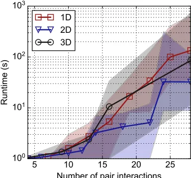
FIG. 4. Single-core computation time needed to find and prove the ground state of a 1D, 2D, and 3D pair-interaction Hamiltonian for unit cells up to 50 sites in size across an increasing range of pair-interactions. In all cases, the solver finds the ground state for all unit cells up to 50 atoms in size and calculates a tight lower bound on the true ground state energy without enlarging|B|. Each point corresponds to the geometric average runtime of 100 such calculations with random interaction coefficients, while the shading gives the spread between the 20th and 80th percentiles.
Nonetheless, we must emphasize that this argument remains a speculation on the convergence behavior, and we are unable to prove convergence beyond 1r. Thus, most generally, we refer to our earlier proof that our method converges at least as quickly and is at least as rigorous as the configura-tional polytope method, while offering definite computaconfigura-tional advantages by means of the MAX-SAT column-generation oracle.
D. Computational performance
To test the performance of this approach on practically relevant systems, we measure the runtime of our algorithm on binary 1D, 2D square, and three-dimensional (3D) cubic lattices over random sets of ECIs across a spectrum of interaction ranges. First, we restrict ourselves to only pair interactions, calculating runtimes for up to 28 pair interactions on unit cells with up to 50 sites, where the energy of each interaction takes on a random value. In the 1D, 2D, and 3D cases, this limit corresponds to all interactions up to and in-cluding the 28th, 10th, and 5th nearest neighbors, respectively. The results of these calculations on a single Intel E5-1650 3.20 GHz core are given in Fig. 4. It is important to note that the code performance could be significantly improved by parallelization—the upper-bound implementation is perfectly parallelizable up to at least hundreds of compute cores, and the lower-bound calculation parallelizes favorably based on the method chosen for the nonsmooth convex optimization.
The results reveal that the primary source of runtime complexity is the range and number of interactions included in the Hamiltonian, with a secondary dependence on the dimensionality of the problem. As could be expected, in-creasing the range of interactions results in an exponential
increase in runtime due to the exponential increase in the size of the spin configuration space. Fortunately, the increase in runtime with the number of interactions at a given range is polynomial. The effect of dimensionality is more subtle: dimensionality determines the number of distinct interactions at a given interaction range, and the number of possible unit cells containing no more than a set number of sites. We find that the former condition is important to the lower-bound calculation runtime, while the latter condition determines the variation in the upper-bound runtime.
In all cases, our implementation gives a very promising single-core runtime on the order of hours for realistic Hamil-tonians, which typically include fewer than 100 interactions. The runtime scales more favorably when all the interactions included in the Hamiltonian are kept below some maximum range—for example, a Hamiltonian with 100 interactions limited to the eighth nearest neighbor range in 3D can be solved in 3 h on a single core. This performance is consistent with the trends presented in Fig.4. In a 3D cubic system, there are 61 pair interactions at or below the eighth nearest neighbor range, which based on the trend in Fig. 4 would indicate a runtime of approximately 104s, or 2.7 h. Thus, if we include
three- and four-body terms in the Hamiltonian, the runtime is comparable to that of a pair-interaction Hamiltonian with the same interaction range.
A curious detail of the runtime data presented in Fig. 4 is that the computation time required for the 1D problem is similar to that of the 3D problem, considering that the number of periodicities is on the order ofO(N) in 1D andO(N3) in 3D,
whereN is the maximum unit cell size under consideration. One qualitative explanation of this behavior relies on the fact that, in our implementation, we first compute the lower bound on energy, and then attempt to converge the upper bound. Given a fixed number of pair interactionsM, the convex optimization in the lower-bound calculations hasDim(λ)=O(M√D
M) for aDdimensional system. Therefore, we may expect that the lower-bound calculation is more expensive in 1D than in 3D at a fixed number of interactionsM. Furthermore, we find that, in 3D, we are often able to terminate the upper-bound calculation quickly as it converges to the lower bound at a relatively small periodicity, foregoing the general O(N3) MAX-SAT
calculations. One possible explanation of this behavior relates to the fact that we measure problem complexity by the number of interactions rather than their range. Consequently, in 3D, theMinteractions are more mutually exclusive in relation to 1D as they are confined to a much shorter range, reducing the effective number of interactions relevant to the solution.
E. Application to a realistic Hamiltonian
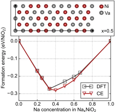
Finally, we apply our method to obtain the exact ground state of a cluster expansion Hamiltonian used to model sodium-vacancy orderings in the layered NaxNiO2 compound as a
0.0 0.2 0.4 0.6 0.8 1.0 Na concentration in NaxNiO2
−0.3 −0.2 −0.1 0.0 0.1
F
or
m
ation
energy
(eV/NiO
2
)
DFT CE
Ni Va
[image:11.608.76.270.70.260.2]x=0.5
FIG. 5. Ground states found for a cluster expansion Hamiltonian of sodium-vacancy orderings in layered NaxNiO2. The red triangles indicate the mathematically proven ground states of the lattice model, whereas the gray squares are the originally proposed ground states from DFT calculations of 400 possible Na-vacancy arrangements. The ground state configuration forx=1/2 is shown in the inset. configurational polytope method [32,33], a LP system with about 232 variables and 232 constraints would be required to
capture the frustration effect necessary to provide a tight lower bound. Such a LP system cannot be solved in a practically relevant amount of time. In contrast, our method not only finds the exact ground states, but also proves their optimality on a timescale of minutes to hours.
As can be observed in Fig.5, our algorithm finds ground states at x=2/5,1/2, and 3/5 that were not within the set of DFT input structures initially used to derive the cluster expansion. As we are able to prove that the solutions are optimal, we can guarantee that there are no other configurations that are lower in energy. The inset shows the unusual ground state predicted atx=1/2, which is unlikely to be proposed from intuition.
V. CONCLUSION
We have introduced a computationally efficient and math-ematically rigorous MAX-MIN procedure which is, in many
cases, able to obtain the exact ground state of a generalized Ising model and prove its optimality both within a constrained periodicity and with respect to all possible periodicities. To the best of our knowledge, our approach is the only known method of approaching the problem of proving exact ground states of generalized Ising Hamiltonians with interactions of practically relevant complexity. In developing our procedure, we have derived an efficient approach to find an upper bound on the energy by transforming the finite optimization into a Boolean problem in the form of MAX-SAT, which provides a provable periodically constrained optimum for the Hamiltonian. We also derived a lower bound on the energy from convex optimization over translationally equivalent clusters. We then converged the upper and lower bounds on the energy to attempt to prove the global optimality of the periodic ground state.
We find that our method is formally related to the most rigorous form of the traditional configurational polytope method, but provides a practical approach for handing the generally exponential number of variables and constraints. Thus, while we are unable to guarantee a provable global ground state solution in all cases, we are able to (1) find and prove a periodically constrained ground state up to a predetermined unit cell size, (2) guarantee global optimality in certain cases, and (3) guarantee accuracy at least at the level of the most rigorous configurational polytope method, while offering numerous advantages in terms of computational efficiency. We demonstrate that, in practice, our procedure performs very well and has made it possible to determine the exact ground states of many formerly intractable systems, e.g., the cluster expansions of battery systems.
ACKNOWLEDGMENTS
This paper was supported primarily by the US Department of Energy (DOE) under Contract No. DE-FG02-96ER45571. In addition, some of the test cases for ground states were supported by the Office of Naval Research under contract N00014-14-1-0444. Additionally, the authors thank Stephen Boyd, Asu Ozdaglar, and Juan Pablo Vielma for inspiration on convex optimization. We are grateful to Joseph O’Rourke and Joel David Hamkins for guidance on tiling and complex-ity theory. Further, we thank Carlos Ans´otegui, Dr. Josep Argelich, and Dr. Adrian Kuegel for kindly providing us different MAX-SAT solvers.
[1] X. Li, X. Ma, D. Su, L. Liu, R. Chisnell, S. P. Ong, H. Chen, A. Toumar, J.-C. Idrobo, Y. Lei, J. Bai, F. Wang, J. W. Lynn, Y. S. Lee, and G. Ceder,Nat. Mater.13,586(2014).
[2] G. D. Garbulsky and G. Ceder,Phys. Rev. B51,67(1995). [3] J. Struck, M. Weinberg, C. ¨Olschlager, P. Windpassinger, J.
Simonet, K. Sengstock, R. H¨oppner, P. Hauke, A. Eckardt, M. Lewenstein, and L. Mathey,Nat. Phys.9,738(2013).
[4] C. K. Aidun and J. R. Clausen,Annu. Rev. Fluid Mech.42,439 (2010).
[5] T. Mueller and G. Ceder,Phys. Rev. B74,134104(2006). [6] K. Kremer and K. Binder,Comput. Phys. Rep.7,259(1988).
[7] A. Seko, K. Yuge, F. Oba, A. Kuwabara, and I. Tanaka,Phys. Rev. B73,184117(2006).
[8] D. H. Rothman and S. Zaleski,Lattice-Gas Cellular Automata: Simple Models of Complex Hydrodynamics(Cambridge Univer-sity Press, Cambridge, 2004), Vol. 5.
[9] A. van de Walle,Nat. Mater.7,455(2008).
[10] A. Van der Ven and G. Ceder,Phys. Rev. B71,054102(2005). [11] F. Casola, T. Shiroka, S. Wang, K. Conder, E. Pomjakushina, J.
Mesot, and H. R. Ott,Phys. Rev. Lett.105,067203(2010). [12] J. M. Sanchez, F. Ducastelle, and D. Gratias,Phys. A
[13] U. Frisch, B. Hasslacher, and Y. Pomeau,Phys. Rev. Lett.56, 1505(1986).
[14] W. Li, J. N. Reimers, and J. R. Dahn,Phys. Rev. B46,3236 (1992).
[15] M. K. Y. Chan, J. Reed, D. Donadio, T. Mueller, Y. S. Meng, G. Galli, and G. Ceder,Phys. Rev. B81,174303(2010).
[16] E. Ising,Z. Physik31,253(1925).
[17] G. Ceder,Comput. Mater. Sci.1,144(1993).
[18] Y. Hinuma, Y. S. Meng, and G. Ceder,Phys. Rev. B77,224111 (2008).
[19] V. Ozoliņˇs, C. Wolverton, and A. Zunger,Phys. Rev. B57,6427 (1998).
[20] M. Asta and V. Ozoliņˇs,Phys. Rev. B64,094104(2001). [21] B. P. Burton and A. van de Walle,Calphad37,151(2012). [22] F. Zhou, T. Maxisch, and G. Ceder,Phys. Rev. Lett.97,155704
(2006).
[23] Y. I. Dublenych,Phys. Rev. Lett.109,167202(2012). [24] Y. I. Dublenych,Phys. Rev. E84,011106(2011). [25] Y. I. Dublenych,Phys. Rev. E84,061102(2011). [26] M. Teubner,Phys. A (Amsterdam, Neth.)169,407(1990). [27] J. Kanamori and M. Kaburagi, J. Phys. Soc. Jpn. 52, 4184
(1983).
[28] M. Kaburagi and J. Kanamori,J. Phys. Soc. Jpn.44,718(1978). [29] A. Finel and F. Ducastelle,Europhys. Lett.1,135(1986). [30] E. Aarts and J. Korst, Simulated Annealing and Boltzmann
Machines(John Wiley and Sons Inc, New York, 1966). [31] N. Metropolis, A. W. Rosenbluth, M. N. Rosenbluth, A. H.
Teller, and E. Teller,J. Chem. Phys.21,1087(1953).
[32] F. Ducastelle, Order and Phase Stability in Alloys (North-Holland, New York, 1991).
[33] M. Kaburagi and J. Kanamori,Prog. Theor. Phys.54,30(1975). [34] D. D. Fontaine, Solid State Phys.47, 33 (1994).
[35] G. D. Garbulsky, P. D. Tepesch, and G. Ceder, in MRS Proceedings(Cambridge University Press, Cambridge, 1992), p. 259.
[36] G. Ceder, G. D. Garbulsky, D. Avis, and K. Fukuda,Phys. Rev. B49,1(1994).
[37] https://github.com/dkitch/maxsat-ising.
[38] P. A. Graf, K. Kim, W. B. Jones, and G. L. W. Hart,Appl. Phys. Lett.87,243111(2005).
[39] A. F. Kohan, P. D. Tepesch, G. Ceder, and C. Wolverton, Comput. Mater. Sci.9,389(1998).
[40] Y. Zhang, V. Ozolins, D. Morelli, and C. Wolverton, Chem. Mater.26,3427(2014).
[41] A. Van der Ven, M. K. Aydinol, G. Ceder, G. Kresse, and J. Hafner,Phys. Rev. B58,2975(1998).
[42] G. L. W. Hart and R. W. Forcade,Phys. Rev. B 77, 224115 (2008).
[43] D. G. Luenberger, Introduction to Linear and Nonlinear Programming(Addison-Wesley Reading, Boston, MA, 1973), Vol. 28.
[44] R. S. Garfinkel and G. L. Nemhauser,Integer programming
(Wiley, New York, 1972), Vol. 4.
[45] E. Boros and P. L. Hammer,Discrete Applied Mathematics123, 155(2002).
[46] C. Ans´otegui, M. L. Bonet, and J. Levy, inTheory and Appli-cations of Satisfiability Testing-SAT 2009(Springer, Swansea, 2009), p. 427.
[47] C. Luo, S. Cai, W. Wu, Z. Jie, and K. Su,IEEE Trans. Comput.
64,1830(2015).
[48] C. P. Gomes, H. Kautz, A. Sabharwal, and B. Selman,Handbook of Knowledge Representation3,89(2008).
[49] J. Argelich, C.-M. Li, F. Manya, and J. Planes, Journal on Satisfiability, Boolean Modeling and Computation4, 251 (2008).
[50] C. Ans´oTegui, M. L. Bonet, and J. Levy,Artif. Intell.196,77 (2013).
[51] H. H. Hoos and T. St¨utzle,Stochastic Local Search: Foundations and Applications(Elsevier, Amsterdam, 2004).
[52] T. St¨utzle, H. Hoos, and A. Roli, Rapport Technique AIDA-01-02, Intellectics Group, Darmstadt University of Technology, Germany (2001).
[53] A. K¨uegel, inLearning and Intelligent Optimization(Springer, Berlin, 2012), p. 431.
[54] S. P. Boyd and L. Vandenberghe,Convex Optimization (Cam-bridge University Press, Cam(Cam-bridge, 2004).
[55] K. C. Kiwiel,SIAM J. Control34,660(1996).
[56] K. C. Kiwiel,Mathematical Programming46,105(1990). [57] H. Wang,Bell Syst. Tech. J.40,1(1961).
[58] R. M. Robinson,Invent. Math.12,177(1971).
[59] R. Berger,The Undecidability of the Domino Problem (Ameri-can Mathematical Society, Providence, 1966).
[60] D. Bertsimas and J. N. Tsitsiklis, Introduction to Linear Optimization(Athena Scientific Belmont, Belmont, MA, 1997), Vol. 6.
[61] A. van de Walle, The effect of lattice vibrations on substitutional alloy thermodynamics, Ph.D. thesis, Massachusetts Institute of Technology, 2000.
[62] W. Huang, D. Kitchaev, S. Dacek, Z. Rong, Z. Ding, and G. Ceder,arXiv:1606.07429(2016).