Galactic microlensing : binary lens light curve morphologies and results from the Rosetta spacecraft bulge survey

GALACTIC MICROLENSING

BINARY-LENS LIGHT CURVE MORPHOLOGIES AND

RESULTS FROM THE ROSETTA SPACECRAFT BULGE

SURVEY

Christine Elisabeth Liebig

A Thesis Submitted for the Degree of PhD at the

University of St Andrews

2014

Full metadata for this item is available in Research@StAndrews:FullText

at:

http://research-repository.st-andrews.ac.uk/

Please use this identifier to cite or link to this item:

http://hdl.handle.net/10023/4881

This item is protected by original copyright

Galactic Microlensing

Binary-lens light curve morphologies and

results from the Rosetta spacecraft bulge survey

Christine Elisabeth Liebig

Submitted for the degree of

Doctor of Philosophy in Astronomy

Declaration

I, Christine Liebig, hereby certify that this thesis, which is approximately 20.000 words in

length, has been written by me, that it is the record of work carried out by me and that it

has not been submitted in any previous application for a higher degree.

Date Signature of candidate

I was admitted as a research student in January 2010 and as a candidate for the degree of

PhD in January 2010; the higher study for which this is a record was carried out in the

University of St Andrews between 2010 and 2013.

Date Signature of candidate

I hereby certify that the candidate has fulfilled the conditions of the Resolution and

Reg-ulations appropriate for the degree of PhD in the University of St Andrews and that the

candidate is qualified to submit this thesis in application for that degree.

Date Signature of supervisor

Copyright Agreement

In submitting this thesis to the University of St Andrews we understand that we are

giv-ing permission for it to be made available for use in accordance with the regulations of

the University Library for the time being in force, subject to any copyright vested in the

work not being affected thereby. We also understand that the title and the abstract will be

published, and that a copy of the work may be made and supplied to any bona fide library

or research worker, that my thesis will be electronically accessible for personal or research

use unless exempt by award of an embargo as requested below, and that the library has

the right to migrate my thesis into new electronic forms as required to ensure continued

access to the thesis. We have obtained any third-party copyright permissions that may be

required in order to allow such access and migration, or have requested the appropriate

embargo below.

The following is an agreed request by candidate and supervisor regarding the electronic

publication of this thesis:

Access to Printed copy and electronic publication of thesis through the University of St

Andrews.

Date Signature of candidate

Date Signature of supervisor

Abstract

For 20 years now, gravitational microlensing observations towards the Galactic bulge have provided us with a wealth of information about the stellar and planetary content of our Galaxy, which is inaccessible via other current methods. This thesis summarises work on two research topics that arose in the context of exoplanetary microlensing, but we take a step back and consider ways of increasing our understanding of more fundamental phenomena: firstly, stellar microlenses in our Galaxy that were stereoscopically observed and, secondly, the morphological variety of binary-lens light curves.

In autumn 2008, the ESA Rosetta spacecraft surveyed the Galactic bulge for microlensing events. With a baseline of ∼1.6 AU between the spacecraft and ground observations, significant parallax effects can be expected. We develop a photometry pipeline to deal with a severely undersampled point spread function in the crowded fields of the Galactic bulge, making use of complementary ground observations. Comparison of Rosetta and OGLE light curves provides the microlens parallax πE, which constrains the mass and

distance of the observed lenses. The lens mass could be fully determined if future proper motion measurements were obtained, whereas the lens distance additionally requires the determination of the source distance.

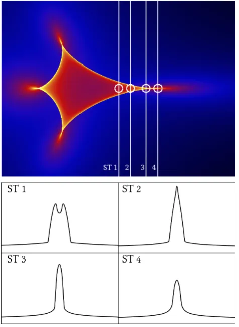
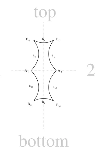
In the second project, we present a detailed study of microlensing light curve morpholo-gies. We provide a complete morphological classification for the case of the equal-mass binary lens, which makes use of the realisation that any microlensing peak can be cat-egorised as one of only four types: cusp-grazing, cusp-crossing, crossing or fold-grazing. As a means for this classification, we develop a caustic feature notation, which can be universally applied to binary lens caustics. Ultimately, this study aims to refine light curve modelling approaches by providing an optimal choice of initial parameter sets, while ensuring complete coverage of the relevant parameter space.

Contents

Abstract 7

Table of Contents 10

I Galactic gravitational microlensing

11

1 Gravitational lensing 13

2 Microlensing fundamentals 17

2.1 Lens equation . . . 17

2.2 Einstein ring . . . 20

2.3 Lens magnification . . . 21

2.4 Paczyński curve . . . 22

2.5 Single lens events . . . 23

2.6 Multiple lenses . . . 24

2.7 Higher-order effects . . . 26

2.8 Modelling . . . 28

3 Exoplanetary microlensing 31

II Rosetta bulge microlensing campaign

35

5.2 Analysis . . . 43

5.3 Limitations of the photometric analysis . . . 48

6 Microlens parallax 51

10 CONTENTS

7 Results 57

7.1 Rosetta microlensing events . . . 57

7.2 Paczyński fit . . . 57

7.3 Microlens parallax measurement . . . 60

7.4 Physical properties . . . 61

8 Conclusion and future prospects 63

III Morphology of binary-lens light curves

65

10.2 Notation for binary-lens caustic features . . . 81

11 Methodology 87 11.1 Light curve simulation and processing . . . 87

11.2 Iso-maxima regions . . . 88

12 Results 93 12.1 Classes overview . . . 96

12.2 Further considerations . . . 102

13 Conclusion and future prospects 107 14 Appendix Morphology 109 14.1 s = 0.65 . . . 109

14.2 s = 0.7 . . . 112

14.3 s = 0.85 . . . 115

14.4 s = 1.0 . . . 118

14.5 s = 1.5 . . . 121

14.6 s = 2.05 . . . 124

14.7 s = 2.5 . . . 127

Part I

Introduction to gravitational

microlensing towards the Galactic bulge

1

|

Gravitational lensing

Gravitational lensing occurs when the light of a background source is deflected by an

in-tervening massive body. This phenomenon can be observed on all astronomical scales. At

the cosmological distance scale, quasars are gravitationally lensed by foreground

galax-ies, and early galaxies are lensed by galaxy clusters. In the Local Group, we can detect

star-on-star lensing. In the phenomenon named “strong lensing” single or multiple images

of the same source can be observed that will be more or less distorted from their

origi-nal shape. A single point-mass lens acting on a single background source will create an

Einstein ring (Figure 1.1), if source, lens and observer are perfectly aligned, but if that is

not the case it always produces two (distorted) images of the background source, one

out-side and another one, mirror-inverted and flipped, inout-side the imaginary Einstein ring. As

long as the angular distance between the source and the lens is substantially larger than

the Einstein ring radius, the inner image will be vanishingly small and the outer image

matches the unlensed source. But if the angular separation is of the order of the Einstein

radius or smaller, then the inner image will increase in size and the centroid of the outer

image is increasingly shifted away from the projected source position. In “microlensing”

the images cannot be resolved in normal observations, simply because the angular scale

is so much smaller in Galactic gravitational lensing with an Einstein ring size of the

or-der of milliarcseconds rather than arcseconds (Figure 1.2)1. Because of this, star-on-star

lensing is next to impossible to discover in static systems2_{. But transient events that}

oc-cur whenever there is a relative transverse movement of source and lens can be detected

1_{Microlensingdoeshappen in the extragalactic setting as well, when the macro images of a quasar pass}

through a dense stellar field of the lensing galaxy and individual stars act as (secondary) lenses.

2_{As Einstein (1936) put it: “no great chance of observing this phenomenon”.}

14

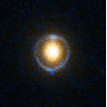
Figure 1.1: Hubble ACS B- and I-band image of gravitational lens SDSS J232120.93-093910.2. The light of a (blue) background galaxy is de-flected by the (yellow) foreground galaxy to form the Einstein ring. The image is 8 arcsec-onds wide.

Credit: NASA, ESA, A. Bolton

(Harvard-Smithsonian CfA) and the SLACS Team.

as a passing increase in brightness. A single point-mass lens is then detected through a

symmetric rise and fall in flux; the light curve can be expressed in a strictly analytic form.

The fundamental equations of gravitational lensing are discussed in Chapter 2. The lens

system can be more complex: exoplanetary research (Chapter 3) is interested in cases that

are composed of a host star with one or more planetary companions. Due to the unique

way that multiple lenses manifest themselves in extended “caustic” structures (imaginary

lines, where the background source star is formally infinitely magnified), the detection of

extrasolar planets via microlensing does not depend on the brightness of their host star

and is sensitive to planets in icy orbits (several AU) around distant (several kpc) host stars.

With extrasolar planets having been detected in their hundreds since the first exciting

dis-coveries in the 1990’s, exoplanetary microlensing might not be leading the numbers game,

but is the method uniquely suited to fill in the parameter space of distant, cool and even

solivagant planets (Gould et al., 2010; Gaudi, 2012; Cassan et al., 2012; Sumi et al., 2011).

Only by combining all available methods, we will be able to gain a full picture of the

planetary population of the Milky Way (Dominik et al., 2008).

While the principal mechanisms of microlensing are well understood, the method still

poses unsolved challenges. Even for the single lens, one cannot directly obtain a full

so-lution, as the physical parameters of the lensing system are all contained within a single

observable, the event duration. In Part II, we can measure a second independent

CHAPTER 1. GRAVITATIONAL LENSING 15

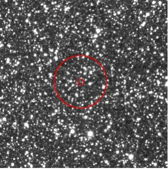
Figure 1.2: Microlensing target OGLE-2008-BLG-510, marked with two red concentric circles, in a typical bulge field. I-band image taken with the DFOSC instrument on the Danish 1.54m tele-scope at ESO La Silla, Chile. The image is 200 arcseconds wide.

Own observation for MiNDSTEp.

binary lens, the transient magnification cannot be expressed in a closed analytical form.

The model optimisation has to work on a highly non-linear parameter space, while each

individual model evaluation is time-costly because typically hundreds of data points from

different telescopes have to be fitted. Modelling the physical characteristics of an observed

lens system often runs into competing solutions; it is essential to increase our

under-standing of the parameter space and the topography of the optimisation surface, which is

2

|

Microlensing fundamentals

2.1 Lens equation

From Einstein’s general theory of relativity (Einstein, 1916) it follows that light is deflected

by massive bodies or, more precisely, that light always follows the null geodesics of

space-time, but spacetime is bent under the influence of gravitation. General relativity predicts

that a light ray which passes a point mass M at a minimum distance ξ will be deflected by

an angle

˜

α = 4GM

c2_ξ , (2.1)

where G denotes the Gravitational constant, c the speed of light. The deflection angle was

first confirmed by Dyson, Eddington & Davidson (1920) during the solar eclipse in 1919,

when they observed the apparent astrometric shifts of the positions of the bright stars of

the Hyades cluster caused by the mass of the sun.

The point mass or point lens approximation is justified in a Galactic lensing situation,

where slowly rotating and nearly spherical stars align to form a gravitational lens system,

assuming that all light rays from the source star pass at a distance from the centre of the

lensing body which is larger than the radius of that body. We can also make the thin-lens

approximation: since the length of the optical system is much larger than the extent of the

lensing body along the line of sight, it is safe to approximate the action of deflection as

instantaneous and as taking place in an imaginary plane at the location of the lensing mass,

the so calledlens plane. The hyperbolic light paths can then be approximated as straight

18 2.1. LENS EQUATION

lines with a sharp bend at the lens plane. We apply these considerations in Figure 2.1.

The gravitational lensing of a single source by a point mass will generally result in

two images of the source. In Galactic stellar microlensing scenarios these arc-shaped

im-ages will be within a milliarcsecond or so of each other and generally photometrically

detected as an apparent amplification of the background source light. Astrometric stellar

microlensing, by means of measuring the light source centroid shift that is caused by the

asymmetric geometry of the two images, has also been proposed. Promising impending

events have been identified by Sahu et al. (2014)1_{and by Proft, Demleitner & Wambsganss}

(2011)2, but the effect has not yet been observed in practice. In the Galactic context, we

most commonly observe bulge stars “lensed” by other bulge or disk stars, which sometimes

reveal themselves to be in binary systems and/or hosting planets. This kind of star-on-star

lensing is – with today’s methods – only detected in transient events, where source and

lens star have a non-zero relative proper motion µLS.

If one considers the geometry of Figure 2.1, one can directly infer the lens equation

βDS= θDS–αD˜ LS. (2.2)

The the small-angle approximation, tan x ≈ x, is applied here – justified by the fact that

˜

α, β, θ 1 in (almost) all astronomical settings, with the notable exception of black-hole lensing where the deflection angle can be large, see Bozza (2010a).

Using thescaled deflection angle(i.e. scaled to theobserver plane),

α =˜αDLS DS

, (2.3)

the lens equation can be written as

β = θ – α. (2.4)

1_{Two Proxima Centauri events, measurable later this year with HST’s single-observation∼0.2 mas}

pre-cision.

CHAPTER 2. MICROLENSING FUNDAMENTALS 19

DLS

DS

DL

observer plane lens plane source plane

L ξ

˜

α

η S

β α

θ

I1

O I2

Figure 2.1: Sketch of a gravitational lensing system. The light of a background source S at a distance DSis deflected by the angle ˜α as it follows the null geodesic in the spacetime, curved

by the lensing mass L at a distance DL, before it reaches the observer O. The light path is shown

in the thin-lens approximation, with a sharp bend at the lens plane, not in the true hyperbolic form. I1 and I2denote the apparent locations of the two images of the source. For the observer’s

20 2.2. EINSTEIN RING

It is a mapping _R2 7→ _R2_{, from the lens plane to the source plane. The apparent source}

position (i.e. the image position) θ maps to the true source position β. Knowing the

image position θ, the lens equation can be solved for the source position β for any given

mass distribution in the lens plane. Problematic is the inversion of the lens equation.

Determining the image positions θi for a given source position β can, in general, not be

done analytically.

2.2 Einstein ring

If observer, lens and source are perfectly aligned, the two images merge into oneEinstein

ringas the angular source position becomes β = 0.

I2

L S

I1

Figure 2.2:View of the lens plane from the observing point O. The source S is not directly visible and is only depicted here to mark the true source position in rela-tion to the images Ii(see also Figure 2.1). The

(theoret-ical) Einstein ring is indicated by the dashed circle. If the angular separation between L and S is decreased, the two images will further elongate into arcs and fol-low the Einstein ring more closely. If the source is di-rectly behind the lens, the two images merge into one ring-shaped image. Figure reproduced from Paczyński (1996).

With the minimum distance ξ = θDL, we can rewrite the lens equation 2.4,

β = 0 = θ –4GM c2_θ

DLS

DLDS

(2.5)

and solve for the angularEinstein radius,

θE =

r

4GM c2

DLS

DLDS

= s 4GM c2 1 DL – 1 DS , (2.6)

where in the non-cosmological distance scale of our galaxy DLS = DS– DL holds true.

More than being just a singularity, the Einstein radius θEdetermines the angular scale

CHAPTER 2. MICROLENSING FUNDAMENTALS 21

restricted to the point mass lens) in terms of the Einstein radius:

β = θ –θ

2 E

θ (2.7)

This equation has two solutions corresponding to the two images of the source (Figure

2.2),

θ1,2 =

1 2

β±pβ2_{+ 4θ}2 E

. (2.8)

2.3 Lens magnification

The magnification A of an image is defined as the ratio between the solid angle of the

magnified image and the solid angle of the original source,

A = θ β

dθ

dβ, (2.9)

in other words, the ratio of the two-dimensional image and source areas as seen by an

observer.

Since the surface brightness is conserved in the gravitational lensing process (because

of Liouville’s theorem, cf. Misner, Thorne & Wheeler (1973), p. 586), the increased image

area equals an magnification in source brightness when integrating over the image. In

microlensing, where the images are not resolvable by definition, one can only detect the

total brightness magnification changing over time. Substituting β from Equation (2.7) and

employing the useful dimensionless quantity u, defined as the angular separation of the

source from the lens in units of the Einstein angle,

u = β θE

22 2.4. PACZYŃSKI CURVE

two solutions for the two images arise:

A1,2 =

1 –

θE

θ1,2

4–1

= 1 2 ±

u2_{+ 2}

2u√u2_{+ 4}. (2.11)

One image will always lie inside the Einstein ring. In Figure 2.1, this is I2, leading to a

negative impact parameter and formally negative magnification, θ2 < θE ⇒ u2 < 0 ⇒

A2 < 0. The image I2has negative parity with respect to the source, i.e. it appears mirrored

and flipped. While the formal sum of the two magnifications thus is unity, A1 + A2 = 1,

the total flux magnification of the source is obtained by summing over the two absolute

values,

A = |A1| + |A2| =

u2+ 2

u√u2_{+ 4}. (2.12)

If the source is located at an angular separation from the lens of exactly one Einstein angle,

β = θE ⇔u = 1, the total magnification will become,

A(β = θE) =

3

√

5 ≈1.34. (2.13)

Translating this (dimensionless) magnification of the source flux into the apparent

bright-ening compared to the unlensed source in magnitudes viamag = –2.5 log₁₀A, this

corre-sponds to an increase in brightness of ∆mag= –0.32.

2.4 Paczyński curve

If the relative projected positions of a point-mass lens and a point source star change over

time and under the assumption that they move uniformly and on rectilinear paths, the

angular lens-source separation can be parameterised as a function of time,

u(t) =

s

u2 0+

t – t0

tE

2

CHAPTER 2. MICROLENSING FUNDAMENTALS 23

where u0 is the impact parameter, i.e. the separation angle at the time t0 of closest

ap-proach. The Einstein time tE is the time it takes the source to cross the Einstein radius

(tE= θE/µLS), providing a characteristic time scale for an individual transient event.

Plug-ging u(t) into Equation (2.12) gives the time dependent magnification,

A(t) = u(t)

2_{+ 2}

u(t)pu(t)2_{+ 4}, (2.15)

corresponding to the magnitude variation (∝ log A(t)) in the plot on the right-hand side of Figure 2.3. This function is known as the point-source, point-lens (PSPL) light curve

or the Paczyńskicurve as it was first shown in Paczyński (1986). In Equation (2.15) the

magnitude variation is only dependent on the one parameter u, which itself is a function

of t, t0 and tE.

Brightness

Time

Figure 2.3:If a source star passes behind a lens star (centre) along the source trajectory depicted in the magnification map on the left, this gives rise to a point-source, point-lens light curve, also calledPaczyński curve, following the analytic form of Equation (2.15).

2.5 Single lens events

Light curves such as the one in Figure 2.3 can be observed in star-on-star lensing and

24 2.6. MULTIPLE LENSES

survey the Galactic bulge, such as OGLE3 and MOA4, although the probability for an

individual event is only “one in a million” (Paczyński, 1986; Griest, 1991).

The single-lens light curve is observed as the magnified source star flux FS, which can

be blended with unmagnified flux Fblend from unresolved neighbouring sources (or light

from the lens star itself),

F(t) = A(t)FS+ Fblend = (A(t) + g)FS, (2.16)

where we have A(t) from Equation (2.15) and we introduce the blend factor g = Fblend/FS.

The fluxes FS and Fblend are specific to the observing instrument, because the filter

bandpass and resolution obviously affect the collection of photons from the target and

nearby targets. When data points from different telescopes are combined for the model

search (as is common practice in Galactic microlensing), the number of free parameters is

therefore increased by a pair of [Fi_S, Fi_blend] per instrument and filter.

2.6 Multiple lenses

Much attention in current Galactic microlensing is paid to multiple-lens systems, which

may or may not contain planetary lenses. For the projected positions, which are now

two- rather than one-dimensional, one can use complex coordinates. Let η be the source

position in the lens plane and ξ an image position. For N point-mass lenses the lens

equation then becomes (Witt, 1990; Gaudi, Naber & Sackett, 1998)

η = ξ +

N

X

i=1

q_i ξi– ξ

, (2.17)

where q_i is the mass ratio between lens i and the primary lens (q_i = Mi

M0), which is

conve-niently placed at the origin (ξ0 = 0). The magnification is now obtained as the inverse of

CHAPTER 2. MICROLENSING FUNDAMENTALS 25

the determinant of the Jacobian of the mapping equation (2.17),

A = 1

det J(ξ) with det J(ξ) = 1 –

∂η

∂ξ

∂η

∂ξ. (2.18)

In the case J(ξ) = 0, a hypothetical point source would undergo infinite magnification

(whereas a real, extended source will be highly, but finitely magnified). The mapping

of all image positions satisfying J = 0 (called critical curves) to the source plane forms

caustics, lines of formally infinite magnification that arise when the lens system is not

circularly symmetric or when it is a continuous mass distribution5. Caustic lines offer a

visualisation of the “optics” of a gravitational lens system.

In Figure 2.4, we see a magnification map with caustic structures and an extracted light

curve, while Figure 2.5 shows the three topologies of binary lens caustics.

Brightness

Time

Figure 2.4:Caustics form when there an asymmetric lens mass distribution, for example, several point lenses. The magnification map, on the left, corresponds to a star-planet binary, with a mass ratio of 10–3. If the source trajectory crosses the caustic lines, this often gives rise to a characteristic deviation from the Paczyński curve, a binary signature.

The multiple lens case is much more complex than the single lens case that we looked

at before. The simple quadratic form of Equation (2.7) now gives way to a fifth-order

polynomial with 3 solutions, or 5 if the source is inside the caustic lines, in the case of a

binary lens (Schneider & Weiß, 1986), whereas for a triple lens the polynomial is already

5_{For a single point lens, the “caustic” is a single point at the position of the lens and the Einstein ring is}

26 2.7. HIGHER-ORDER EFFECTS

of 10th order with 4 up to 10 solutions, where an extra pair is created or destroyed at

every caustic crossing (Rhie, 1997). The number of solutions corresponds to the number

of images of the source. While this is theoretically true it can conjure up a misleading

idea: when η → ∞, there are still three images for a binary lens system, one coinciding with the unmagnified source star and the other two at the two lens positions ξi, but with

zero magnification they cannot be seen as physical images. When the source moves closer

to the lens system, the latter two images move away from the lens positions and have a

non-zero photon flux.

2.7 Higher-order effects

2.7.1 Extended source effects

Generally speaking, an extended source will “blur” caustic lines and broaden and flatten

peaks of high magnification. The simple model of a point source can be sufficient for

single-lens cases as long as the minimum angular distance to the lens is at least of the

order of several angular source radii ρ, but it breaks down when an extended source gets

very close to the lens (Gould, 1994a; Witt & Mao, 1994). If the lens is a binary,

extended-source effects become significant whenever the extended-source is close to a caustic line, which is

observed in the majority of binary microlensing events (see, for example, Jaroszyński et al.

(2010)). Night, Di Stefano & Schwamb (2008) however argues that this might eventually

be traced back to a selection effect, as “smoothly-perturbed” binary light curves are much

easier to miss in the data noise.

Events that reach a very high magnification can display chromatic limb-darkening

effects (see, for example, Alcock et al., 1997; Zub et al., 2011).

2.7.2 Microlens parallax

Parallax effects can be detected, when event observations from more than one location

CHAPTER 2. MICROLENSING FUNDAMENTALS 27

and observer breaks down. An example of the latter is the Earth-orbital parallax: the

orbital movement of the Earth around the Solar system barycentre can cause a wave-like

perturbation in long-timescale events with a period of one year with the non-uniform

change in angular lens-source separation,u(t)˙ 6= 0. In medium time-scale events it can still be detected as a significant asymmetry, as in the first detected microlens parallax effect

(Alcock et al., 1995). The same effect on the light curve can be caused by a source star

that is orbiting a binary companion, although it can be assumed that the probability for

it to match the annual period and orientation is low. This latter effect is sometimes called

xallarap, to emphasise that it is a kind of “reverse parallax” effect (Poindexter et al., 2005).

The very steep gradient of caustic crossings sometimes allows to detectterrestrial

par-allaxeffects, when telescopes spread across the globe observe the exact peak of the caustic

crossing at slightly different times due to the (minute) differences in perspective, in effect

“time-shifting” the light curve. The first successful observations of this effect are described

in Gould et al. (2009).

Of course, the effect persists on a larger scale: Earth-spacecraft parallax is the term

commonly used, when two quasi-independent light curves of the same source-lens system

are observed by telescopes that are separated by a baseline of the order of AUs. In Part II

of this work, we discuss observations of this effect and treat the theory of the microlens

parallax in more detail (Chapter 6).

2.7.3 Orbital motion

In most Galactic binary microlensing events, with a typical timescale of tE ∼ 1 month,

orbital motion can be ignored in the modelling, but the longer the duration of the event,

the more likely are perturbations to the static model (Dominik, 1998). The orbital motion

rotates and changes the shape of the binary caustic. This kind of caustic change was

detected in the triple-lens, two-planet system OGLE-2006-BLG-109 and helped to constrain

28 2.8. MODELLING

2.7.4 Binary sources

Smoothly perturbed, i.e. non-caustic-crossing, binary lens light curves can be virtually

indistinguishable from a microlensedbinary source, where the Paczyński curve of the first

source star is followed and superposed by that of its binary companion to give the

im-pression of a smooth double-peaked cusp-grazing light curve as caused by a single source

(Griest & Hu, 1992). Jaroszyński et al. (2010), for example, show competing binary-source

and binary-lens models for many binary events from the 2006-2008 OGLE-III database. In

principle, these can be distinguished by colour effects, which was originally proposed by

Gaudi (1998) and first carried out by Hwang et al. (2013).

2.8 Modelling

Different approaches have been tried out to deal with the fact that the microlensing

mag-nification cannot be analytically calculated for multiple lens systems. One is the inverse

ray-shooting method, where light rays are traced back from the observer to the source

plane, summing up the deflection by individual masses in the lens plane. After deflection,

all light rays are collected in pixels of the source plane. Since this is equivalent to tracing

rays from the background source to the observer plane, the calculated magnification

pat-tern then shows the magnification a pixel-sized source would experience at the respective

pixel position in the source plane. A one-dimensional cut through a magnification map

that has been convolved with a source profile represents a light curve model. The source

model can have an arbitrary shape; here we use a flat-disc model, parametrised by a radius

ρ.

This method was first deployed for microlensing purposes by Schneider & Weiß (1986)

and Kayser, Refsdal & Stabell (1986), and later refined by Wambsganss (1990, 1999) to

accommodate for a large number of lenses. It was first applied to planetary microlensing in

Wambsganss (1997) and various implementations exist (Bennett & Rhie, 1996; Rattenbury

et al., 2002; Dong et al., 2006; Hundertmark, Hessman & Dreizler, 2008), the latest being a

CHAPTER 2. MICROLENSING FUNDAMENTALS 29

The other method is contouring along the source images (Schramm & Kayser, 1987),

in effect applying Green’s theorem to find the image magnification by integrating along

its contours. This method has also been further developed (Dominik, 1995; Gould &

Gaucherel, 1997; Dominik, 1998; Dong et al., 2006; Dominik, 2007; Bozza, 2010b). This

is a method with potentially very fast computing, although this can break down in

high-magnification events, when the image contour becomes comparable in size to the image

30 2.8. MODELLING

(a) Close binary case. Depicted here is an angular separation of d = 0.7θE.

(b) Intermediate binary case. d = 1.0θE.

(c) Wide binary case. d = 1.3θE.

3

|

Exoplanetary microlensing

After centuries of speculation about the existence of worlds apart from our own and many

failed attempts to secure evidence for them (Marcy & Butler, 2000), the recent decades

have finally brought robust detections of extrasolar planets of which hundreds and

thou-sands1 _{have been confirmed to date. There are many excellent introductions to the}

fast-evolving field of exoplanetary research; Perryman (2011) covers the techniques as well as

the breakthrough discoveries, from the first planetary system discovered around a

pul-sar (Wolszczan & Frail, 1992), the first planet around a main-sequence star, detected via

radial-velocity measurements, (Mayor & Queloz, 1995) and the first transit detection of

an extrasolar planet (Henry et al., 2000; Charbonneau et al., 2000), up to a preview of the

state-of-the-art space programmes, the transit monitoring Kepler/NASA2_{which helped to}

almost double the then-known number of exoplanets over its (original mission) lifetime

2009–2013 and Gaia/ESO3_{, launched December 2013, which is designed for astrometry,}

but should have considerable impact on extrasolar planet research not only with its

astro-metric planet detections but also with time-series searches such as microlensing.

Exoplanetary microlensing was first put forth when Liebes (1964) mentioned that

ex-trasolar planets around lensing host stars would perturb the microlensing event light curve

of the stellar lens, but the idea could was not put into practice at the time.

Paczyński (1986) pointed out the possibility of gravitational lensing due to masses as

small as 10–11_M

in the halo of the Milky Way with background source stars in the nearby

1_exoplanet.eu

2_{nasa.gov/kepler}

3_{sci.esa.int/gaia}

32

galaxies4; this minimum mass estimate is limited by the requirement of having an angular

source size which is smaller than the Einstein ring to achieve a significant magnification

(assuming solar-size source stars in the paper). If found, those masses would provide an

explanation of the dark matter in the halo. The idea was eventually picked up and several

searches for microlensing events were called into life in the early 1990s. Alcock et al.

(1993) and Aubourg et al. (1993) reported discoveries towards the Large Magellanic Cloud.

Udalski et al. (1993) found events towards the Galactic bulge. As a general study of lensing

behaviour Schneider & Weiß (1986) had investigated the case of binary point mass lenses.

Paczyński (1991) provided details of lensing by Galactic bulge stars. On this foundation,

Mao & Paczyński (1991) proposed to look for lensing signatures of binary stars and also

extrasolar planets.

The search for massive compact halo object as potential dark matter, was not very

fruitful (see, e.g., Afonso et al., 2003). Microlensing experiments carried out towards the

Galactic bulge had originally been intended as test experiments for the halo surveys, but

Mao & Paczyński (1991) estimated that roughly 10% of the lensing events should show

the signature of a binary companion. It was realised, that through constantly

monitor-ing a very large number of stars one would surely detect binary systems and possibly

planets. Gould & Loeb (1992) qualitatively estimated the fraction of light curves that

would show signs of companions of Jupiter or Saturn mass. Bennett & Rhie (1996) found

that Earth-mass planets are in principle detectable. Wambsganss (1997) provided a

de-tailed study of possible planetary light curve perturbations with different mass-ratio and

angular-separation settings, concluding with the identification of the so-called “lensing

zone” between angular star-planet separations of 0.6 to 1.6 θEthat favours detections,

be-cause the planetary anomalies will settle on the slope of the Paczyński curve – on top of

the ongoing primary lens magnification.

Steady monitoring of the Galactic bulge was realised by different groups, since 1992. As

of 2009, OGLE (The Optical Gravitational Lens Experiment, see Udalski et al. (1992)) and

MOA (Microlensing Observations in Astronomy, see Muraki et al. (1999)) are active survey

CHAPTER 3. EXOPLANETARY MICROLENSING 33

collaborations that complement each other by operating wide-field telescopes in Chile and

New Zealand, respectively. Every season these groups detect microlensing events in their

hundreds. In 2004, they jointly discovered a planet of 1.5 Jupiter masses with an orbit of

∼3 AU, which made history as the first microlensing detected planet (Bond et al., 2004). Already in 1995, a cooperative follow-up strategy had been realised by the GMAN

(Pratt et al., 1995) and PLANET networks (Albrow et al., 1998; Dominik et al., 2002). The

idea behind it was, and still is, to find a compromise between the field-of-view, the

sam-pling rate, the limiting magnitude and the resolution of the targets. The survey groups

OGLE and MOA monitor and publish all (detected) microlensing events. To maximise

the gain, the follow-up community only reacts to events that promise to be interesting

– because it is evolving towards a very high magnification or because it already shows

deviations from the Paczyński curve. Several groups are active in the field of follow-up

observations,5_{although the distinction between survey and follow-up is less clear cut than}

in the past, as the survey telescopes become increasingly fast and the follow-up networks

include more telescopes, freeing more resources for monitoring observations. The common

goal is to get dense time resolution on interesting light curve features to be able to

con-strain a planetary model (or a binary star model, or a source star atmosphere model etc.)

for that light curve. Crucial to the success of these operations is the continuous exchange

of live data during the observing season6 _{that enables fitting of preliminary models and}

thereby tentative predictions about the development of the light curve, to decide about the

priority of observing the given event. This approach has led to further planet discoveries.

Dominik (2010, Table 1) lists 26 planets reported in the microlensing literature up until

31 December 2009, with stronger or weaker evidence for each individual case. Since then

further planet discoveries have been published (Miyake et al., 2011; Muraki et al., 2011;

Batista et al., 2011; Yee et al., 2012; Kains et al., 2013; Poleski et al., 2014), with some

detections probing the “brown dwarf desert” (Bozza et al., 2012; Street et al., 2013) – a

5_{Currently, these follow-up groups are PLANET (planet.iap.fr), MicroFUN}

(www.astronomy.ohio-state.edu/~microfun), RoboNet-II/LCOGT (robonet.lcogt.net) and

MiNDSTEp (www.mindstep-science.org).

6_{The Galactic microlensing season lasts roughly from April to September, the time of year when the}

34

term that Marcy & Butler (2000) coined to describe the paucity of binary companions with

masses in the brown-dwarf range (13–80 MJupiter). Even the detection of extrasolar moons

seems to be within reach (Bennett et al., 2014; Liebig & Wambsganss, 2010). Gaudi (2010)

Part II

Galactic bulge microlensing events as

observed from the Rosetta spacecraft

in 2008

37

For 20 years now, microlensing observations have provided us with a wealth of

infor-mation about the stellar and planetary content of our Galaxy, which is inaccessible via

other current methods. Ground-based observations have brought us far and the lensing

theory is ever-better understood, but it is the nature of the simplest conceivable

single-source, single-lens lensing event to still pose a challenge as the physical parameters of the

lens are heavily convolved in the common observables.

Dual-site microlensing observations with a significant baseline (comparable to the

pro-jected Einstein radius) provide one more independent observable beyond the common

ob-servables of a transient single-source, single-lens event: the microlens parallax πE.

Combining this with either a measurement of the Einstein radius θEor of the relative

lens-source proper motion µLS, it is possible to obtain a mass and a distance measurement

for an object at a distance of the order of kiloparsecs – without requiring prior assumptions

about the type of the lensing body. Measurements like these are necessary for unbiased

Galactic population estimates, which in turn are fundamental for planet abundance

statis-tics.

Before this background, an enterprising idea was realised in 2008: to “borrow” one of

the cameras of the Rosetta spacecraft (Chapter 4) to monitor the Galactic bulge in order to

collect stereoscopic data on Earth-observed microlensing events.

Sahu et al. (2001) were the first to observe a microlensing light curve from space as

part of an M22-monitoring HST campaign. Other space-based (follow-up) light curves

of individual microlensing targets have been published by Dong et al. (2007) and Muraki

et al. (2011), but our work represents the first (and, to our knowledge, only) space survey

of the Galactic bulge microlensing fields and the only one with a substantial baseline of

O(AU). Recently, Gould and Yee have explored the microlens-parallax measuring potential of space telescopes closer to Earth in a string of publications (Gould & Yee, 2012; Gould,

2013; Gould & Horne, 2013; Yee, 2013; Gould & Yee, 2014).

The photometric analysis (Chapter 5) proved challenging, as we are dealing with

crowded-field data taken with a close-imaging camera (rather than a space telescope).

38

the theoretical context of which is given in Chapter 6. The end result of the study,

pre-sented in Chapter 7, relies on ground light curves published by OGLE (Udalski, 2003) for

the detection of microlens parallax effects between ground and space observations.

Clarification The work in Part II will be published as Liebig et al. (2014b) (in prepara-tion). As is the nature of this kind of research, the work relies heavily on previous

collab-orative efforts. I joined the team in 2012 to analyse the Rosetta microlensing data, all prior

planning and all observational work were done without any input from me. Throughout

4

|

Rosetta spacecraft and mission

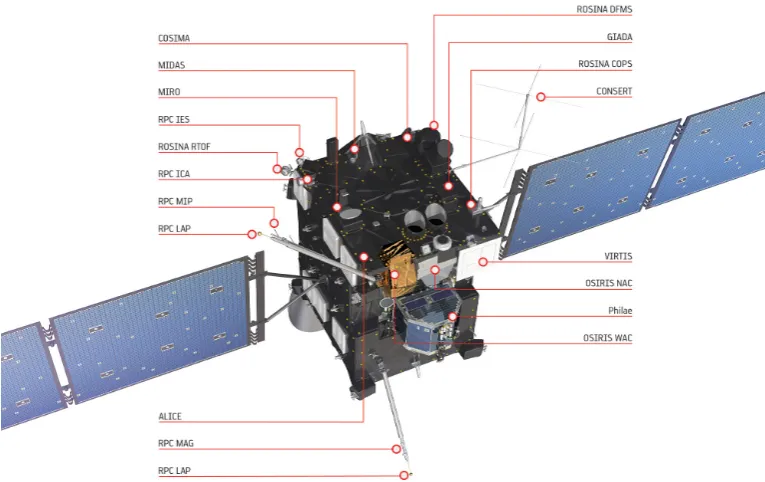
Figure 4.1: Rosetta and its instruments. This study works on data taken by the OSIRIS NAC, where OSIRIS stands for Optical, Spectroscopic, and Infrared Remote Imaging System Camera. OSIRIS is a dual camera imaging system consisting of a narrow-angle (NAC) and a wide-angle camera (WAC) and operating in the visible, near infrared and near ultraviolet wavelength range. Copyright: ESA/ATG medialab

“Rosetta” is one of the cornerstone missions of the European Space Agency. The

space-craft has been launched on 2 March 2004 on a mission to study the comet

67P/Churyumov-Gerasimenko. During its scheduled flight time of 10 years so far, it has completed four

fly-by manoeuvres around Earth and Mars and has had two close encounters with asteroids

2867 Šteins and 21 Lutetia.

Rosetta spent the last 3 years in deep-space hibernation and successfully woke itself

40

up on 20 January 2014 to begin the last leg of its journey. The spacecraft is now being

propelled towards 67P/CG, in May 2014 it will begin a braking manoeuvre to rendezvous

with the comet at a relative speed of 2 m/s in August 2014 and, from then on, it will

continuously monitor the comet on its voyage around the Sun. Rosetta has 11 on-board

instruments, see Figure 4.1, among them OSIRIS (Optical, Spectroscopic, and Infrared

Re-mote Imaging System) dual camera imaging system consisting of a narrow-angle (NAC,

(2◦)2) and a wide-angle camera (WAC, (12◦)2) and operating in the visible, near infrared

and near ultraviolet wavelength range.

Rosetta also carries the “Philae” lander unit with another 14 instruments, which will

be deployed in November 2014 to land on the comet’s surface and examine the chemical

and physical composition of the comet.

The Rosetta microlensing campaign was realised just after the 2867 Šteins flyby in

September 2008 and made use of the OSIRIS Narrow-Angle Camera, originally designed

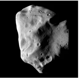
to image asteroids from close range, as shown in Figure 4.2.

Figure 4.2: 21 Lutetia. The asteroid measures about 100 km across and orbits the sun with a semi-major axis of∼

2.4 AU. The image was taken with the OSIRIS Narrow-Angle Camera at closest approach (∼ 3200 km). The surface resolution in this image is approximately 60 meters per pixel.

Copyright: ESA 2010 MPS

for OSIRIS Team

5

|

Photometric analysis of the Rosetta

microlensing data

5.1 Observations

The OSIRIS Narrow-Angle Camera (OSINAC from hereon) observed the Galactic bulge, in

the region [–5◦ < b < –3◦, –5◦ < l < 11◦] in Galactic coordinates, on seven epochs between

7 September and 4 October 2008. On each occasion, eight frames of (2◦)2 were taken. The

OSINAC was designed to image a comet from close range and is not a space telescope.

The pixel scale is 3.9 arcseconds. The diameter of the camera entrance pupil is 89.4 mm.

The “orange” filter was used, as this is the broadband filter with the greatest sensitivity

on-board. For the central wavelength (649.4 nm) of the orange filter, the (purely theoretical)

diffraction limit is 1.82 arcseconds. The uniform exposure time used was 300 seconds. For

all technical specifications of the camera, see Keller et al. (2007a). The data were reduced

using the OSIRIS standard pipeline, the procedure is detailed in e.g. Keller et al. (2007b).

After observations had been concluded, 20 events of interest were identified among the

total of 655 candidate microlensing events announced by the OGLE Early-Warning

Sys-tem1 _{(Udalski et al., 1994) in the 2008 microlensing season. The criteria applied were that}

the candidate event must lie within the OSINAC-covered field, must not last significantly

longer than our observation span (tE < 60 days) and should have peaked reasonably close

to the observing window (7 Sep – tE< t0 < (5 Oct + tE).

For 12 events out of these 20, the team obtained complementary ground observations in

1_{ogle.astrouw.edu.pl/ogle3/ews/2008/ews.html}

42 5.1. OBSERVATIONS

June 2009 using the Wide Field Imager (WFI) instrument mounted on the MPG/ESO

2.2m-telescope, La Silla, Chile (Baade et al., 1999). The filters Rc/162-844 and MB-646/27-8562

were chosen to match the OSINAC orange filter as closely as possible, the passbands are

compared in Figure 5.1. Exposure times were 30 to 45 seconds. The WFI data were reduced

0 0.1 0.2 0.3 0.4 0.5 0.6 0.7 0.8 0.9 1

550 600 650 700 750 800

T ra n sm it ta n ce Wavelength [nm] OSINAC orange WFI MB 867 WFI R 844

Figure 5.1:Passbands of the OSINAC orange filter and the two WFI fil-ters used for follow-up observations. Only observations with the WFI R 844 filter were used in the analysis.

using a version of the Cambridge Astronomical Survey (CASU) pipeline (Irwin & Lewis,

2001) that has been adapted to work with the MPG/ESO WFI instrument. The following

analysis is based on the Rc filter images as they were of an overall cleaner quality, while the

MB data have only been used for sanity checks. Four of these 12 events had to be excluded

from the final analysis, because, back at baseline, they were too faint to be identified on

the WFI frames.

In the end, we have analysed the OSINAC data of eight event candidates, which are

listed in Table 5.1.

CHAPTER 5. PHOTOMETRIC ANALYSIS 43

Event name RA(J2000.0) Dec(J2000.0)

OGLE-2008-BLG-092 17:47:29.42 -34:43:35.6 OGLE-2008-BLG-374 17:54:56.33 -32:50:32.4 OGLE-2008-BLG-517 18:04:16.53 -28:50:22.2 OGLE-2008-BLG-571 18:01:18.75 -30:17:03.2 OGLE-2008-BLG-574 17:56:04.00 -32:05:01.0 OGLE-2008-BLG-582 18:10:24.03 -26:09:05.0 OGLE-2008-BLG-601 18:07:46.78 -26:20:15.0 OGLE-2008-BLG-605 18:07:41.50 -27:25:17.9

Table 5.1: Candidate events for the analysis.

5.2 Analysis

The OSINAC frame resolution is not sufficient for a direct identification of the

microlens-ing targets. This problem is aggravated by the high source density of the observed fields,

Figure 5.2 illustrates this problem.

OSIRIS NAC WFI

Figure 5.2: Juxtaposition of two observed frames, showing the same (97.5 arcsec)2 field centred on the target OB08601, which is marked with the green circle. On the left, a OSIRIS Narrow-Angle Camera sub-frame as observed from the Rosetta spacecraft on 7 September 2008; on the right, a Wide-Field-Imager sub-frame, observed with the 2.2m telescope at ESO La Silla, Chile, on 18 June 2009.

44 5.2. ANALYSIS

analysis for the photometric reduction (Alcock et al., 1999), which is well suited for the

detection of difference flux in crowded fields. Originally, we expected to achieve good

results with a direct image subtraction, because space-based observations are free from

atmospheric perturbations. Unfortunately, image subtraction is not a viable option here,

because the point-spread functions not only change considerably between epochs due to

the spacecraft drift, but are severely undersampled at the same time. Additionally, there

are simply not enough un-crowded stars on the OSINAC frames to calculate the

convolu-tion kernels.

The first challenge was calibrating the astrometry. The OSINAC FITS frames were

fit-ted with initial World Coordinate System (WCS) information using theastrometry.net

code (Lang et al., 2010) and index files based on the USNO-B1.0 catalogue (Monet et al.,

2003), but, due to the aberrations of the optical system, deviations from the true positions

of the order of 10 arcseconds occur on the wide-field frames. We cut down the original

images to 0.125 degree fields, centred on the OGLE candidate events, and repeated the

astrometric calibration. The post-calibration astrometric accuracy of the OSINAC

sub-frames is comparable to the pixel size, i.e. 3.9 arcseconds.

Facing the adverse combination of a low resolution detector and a high stellar density,

as well as a significant pollution with cosmic ray hits, we chose a compromise aperture

size of (3 px)2, where the aperture is placed so that the OGLE target coordinates for the

microlensing event are contained in the central pixel.

The background will generally dominate over the source flux. To separate out the

microlensed flux F from the total aperture flux Faper, we have to subtract the blend flux

Fblend. Since we observed from space, far beyond Earth’s atmosphere, the sky background

is negligible. By visual inspection, we identify and sort out data corrupted by cosmic

ray hits. Afterwards, we consider all non-microlensed flux collected by the aperture as

coming directly from the background stars near the target. These we hoped to identify

from existing ground-based catalogues, but this idea proved to be unfeasible: While the

OGLE photometric catalogue in V and I (Szymański et al., 2011) is cut off too early at

CHAPTER 5. PHOTOMETRIC ANALYSIS 45

for the OSINAC orange filter, the APASS3 catalogue is not deep enough for our purposes

(complete for roughly 10 mag to 17 mag in several filters, of which Sloan r’ is the best

match) and is even more shallow in crowded fields.

Therefore, it was decided to make use of higher-resolution ground observations of the

microlensing events at baseline. In June 2009, when all chosen events of interest were

safely back to baseline, the complementary observations of 12 events were obtained using

WFI.

Using SExtractor (Bertin & Arnouts, 1996), we retrieve a catalogue of WFI sources for

the field of interest around each target, i.e. a data set of sky position and (un-calibrated)

flux {RA, Dec, FWFI}star for each source on the frame. The equatorial coordinates RA and

Dec are converted into the coordinate system of the OSINAC pixels, {X, Y, FWFI}star, to

facilitate the creation of a synthetic OSINAC (baseline) frame. For creating the synthetic

OSINAC frame, we need to photometrically and astrometrically match the WFI catalogue

to the original OSINAC frame, which includes convolving the catalogue stars with the

correct point spread function (PSF). The OSINAC PSF is best described by a Moffat (1969)

function,

PSF(x, y; α, β) = β – 1 πα2

1 +

x2+ y2 α2

–β

. (5.1)

The PSF is severely undersampled in the OSINAC frames with a FWHM of the order of 1

pixel. The flux density for a given source is described by

fWFI(x, y) = FWFI×PSF(x, y; α, β). (5.2)

So we have five parameters to fit: linear shifts δx and δy, the Moffat PSF parameters

α and β and, lastly, a WFI-to-OSINAC flux conversion factor k = F/FWFI. The first four

parameters must be adjusted for each frame, because the stellar PSFs change position and

shape between epochs. The latter parameter, k, on the other hand, should be constant for

a given filter choice (we checked that there was no sensitivity change in the OSINAC CCD

46 5.2. ANALYSIS

over the course of observations). While fitting it, we risk overcompensating for the target

flux variabilities that we want to detect. The fit is also influenced by cosmic ray hits on the

subframe, which are obvious in some cases, but can be imperceptible in others. For these

reasons, we ran the optimisation below on a number of frames withfivefree parameters

until we reached a good match for each frame and then fixed the flux conversion factor at

the mean value, k = 0.1875, leaving onlyfourfree parameters for regular pipeline runs.

We then limit ourselves to a 25×25 pixel OSINAC sub-frame, where the PSF can be assumed stable and the optical aberrations are negligible, and use the SciPy (Jones et al.,

2001–)optimize.fminimplementation of a downhill simplex algorithm to minimise

X

all pixels

FSYN_pixel– Fpixel

p

Fpixel

!2

(5.3)

with the synthetic, WFI-based pixel flux

FSYN_pixel= X

all stars

Z

OSINAC pixel area

fWFI_star ×k, (5.4)

where the stellar flux density is translated by δx, δy and the PSF shape modified by α and

β:

fWFI_star(x – Xstar+ δx, y – Ystar+ δy; α, β). (5.5)

Parameters δx, δy, α, β, are optimised globally over the sub-frame, i.e. a sky area of (97.5

arcsec)2, via Equation (5.3), where typically 0 < |δx| ∼|δy| < 0.5 and α∼1.0, β∼1.5. We can now work on the synthetic frame FSYN_pixel(Figure 5.3, centre) and we are interested in the

synthetic baseline flux.

CHAPTER 5. PHOTOMETRIC ANALYSIS 47

100 1000 10000

100 1000 10000

-800 -400 0 400 800

Figure 5.3: Comparison of the OSINAC frame (left) from Figure 5.2 with its synthetic reproduc-tion from the WFI frame (centre). On the right is the difference image. A cosmic ray from the original image stands out in the top-right quarter and the brighter targets on the lower left of the frame can be traced by their stronger residuals.

in the aperture,

FSYN_aper = X

pixel in aperture

FSYN_pixel(α, β, δx, δy). (5.6)

Thetargetsynthetic aperture flux, i.e. the synthetic baseline flux, is derived analogously to

Equation (5.4) by identifying the target star in the WFI catalogue through astrometry

(clos-est star to OGLE event coordinates) and visual inspection of the finding chart in doubtful

cases:

FSYN_target=

Z

aperture

fWFI_target(α, β, δx, δy)×k. (5.7)

Now, we infer the OSINAC blend flux from the WFI frame by modelling the aperture

blend flux as

FSYN_blend = FSYN_aper– FSYN_target. (5.8)

The OSINAC data points, F, are then determined, after running the above analysisfor

each frame individually, as

48 5.3. LIMITATIONS OF THE PHOTOMETRIC ANALYSIS

where Faperis the raw OSINAC flux and FSYNblendthe synthetically constructed blend flux. F is

the net target flux with any remaining time variability expected to be microlensing (but cf.

limitations in Section 5.3). The reported uncertainties are the propagated Poisson errors of

the raw OSINAC flux and the synthetic blend flux. The Rosetta microlensing light curves

are discussed in Section 7.

For testing the reliability of the method, we have extracted light curves for a selection

of comparison stars around target OB08601, Figure 5.4 shows the results.

5.3 Limitations of the photometric analysis

There might still be additional blending due to either the limited resolution of the WFI

frames or the limited deblending abilities of SExtractor. Typically, a bright lens star could

be the source of such unresolved blend flux. We address this while fitting the Paczyński

curve, see Section 7.2, by making use of the blend parameter as determined by the OGLE

fit solution to the ground-observed microlensing light curve.

Our tool of choice, SExtractor, was not primarily designed for use on crowded stellar

fields, but for the automatic classification of galaxies. We adapted the input parameters

(circular apertures, low deblending threshold), optimising the stellar identification to a

certain extent, but bear in mind that we use and value this tool for its ready usability

and high throughput rather than expecting completely flawless star catalogue results. We

have carefully checked the correct SExtractor identification of the target stars themselves

and argue that for the blend flux determination it is fairly irrelevant whether two close

neighbours are identified as one or two stars given the difference of scale for the WFI and

OSINAC point spread functions.

Of course, ground observations are affected by changing seeing conditions and a high

sky background, therefore the source identification can hardly be perfect and we miss out

on stars fainter than the WFI magnitude limit4_{. Given the respective areas of the OSINAC}

and WFI detectors, 0.092/2.202 = 0.0017, the flux of stars too faint to be identified on the

4_{About 21 R-mag (S/N≥20) in good conditions, for t}

exp= 60 seconds, based on the ESO exposure time

CHAPTER 5. PHOTOMETRIC ANALYSIS 49

(a) Selected comparison stars around target OB08601, picked to match the baseline brightness of the target. FL05 is probably two unresolved sources.

-0.6

-0.4

-0.2

0

0.2

0.4

0.6

4720 4730 4740

M

ag

n

it

u

d

e

d

iff

er

en

ce

JD - 2450000 FL01

FL02 FL03

FL04 FL05 FL06

OB08601

(b) Corresponding light curves, displayed relative to their respective average magnitude. The data points are connected by lines to guide the eye. The uncer-tainties are modelled as Poisson noise. The variation in the target clearly stands out. FL02 had three obvious cosmic ray hits, those epochs have been eliminated from the light curve.

50 5.3. LIMITATIONS OF THE PHOTOMETRIC ANALYSIS

6

|

Microlens parallax

We recall from Section 2.5, Equation (2.16), that a microlensing light curve is observed as

F(t) = A(t)FS+ Fblend = (A(t) + g)FS,

where A(t) is the single-lens microlensing magnification, Equation (2.15).

The light curve F(t) yields only one fit parameter, tE, which contains all available

in-formation on the “optics” of the lensing set up, i.e. the mass M, the distance DL, the source

distance DSand the relative proper motion µLS(Dominik, 2006):

tE=

1 µLS

s

4G c2 M

1 DL

– 1 DS

. (6.1)

The Rosetta microlensing campaign enabled us to add one more independent observable

to determine the physical properties of the lens system, the microlens parallax πE.

Refsdal (1966) was the first to point out the potential of observing Galactic

gravita-tional microlensing events from Earth and a distant spacecraft at (roughly) the same time.

Due to parallactic viewing, the same background source star and foreground lens will,

in general, result in two light curves with different impact parameters and different peak

times for the two observatories (see Figure 6.1). If there is a relative motion between Earth

and the spacecraft, this can additionally lead to a difference in tE. These differences

pro-vide constraints on both the mass and the distance of the microlensing body, which can

otherwise only be assessed through stellar models and statistical arguments.

The term “microlens parallax” only came into use some time later (see, for example,

52

Gould (2000) where it is defined it as πE := AU e

rE , one Astronomical Unit over the physical

lens-plane Einstein ring radius projected back from the source onto the observer plane).

The quantity is intuitively understood as the relative parallax of lens and source star,

πLS = AU_DL –AU_DS, normalised to the Einstein angle θE:

πE=

πLS

θE

. (6.2)

(6.3)

As we will see, πEcan be expressed in terms of the observables ∆t0 and ∆u0. This

deriva-tion is partly following Gould (1994b), with modernised notaderiva-tion.

We pick a coordinate system in the lens plane with right-handed basis vectors (ek,

e⊥) in units of (dimensionless) Einstein angles. The former, ek, is parallel to the

source-lens relative proper motion, µ_LS = µ_L –µ_S. The latter, e⊥, is parallel to the impact axis,

e⊥ k u₀, which in the case of uniform rectilinear relative motion is always orthogonal

to the relative proper motion. We place the origin of the coordinate system at the lens

position. We use this definition of the coordinate system independently of the observer

position; see Figure 6.1 for an overview.

Now, we consider that the transient microlensing magnification in a given

point-source, point-lens scenario depends only on the angular separation of source and lens

|u(t)|. With the chosen coordinate system,u(t) is identical to the source position as well as

the angular lens-source separation in units of Einstein radii. At a time t, for an Earth-based

observer, the source appears to be at position

u⊕

(t) = t – t

⊕

0

tE

×ek+ u⊕₀ ×e⊥, (6.4)

while at the same time, an observer based on the Rosetta spacecraft would see

uR_{(t) =} t – t R 0

tE

CHAPTER 6. MICROLENS PARALLAX 53

This means we have an apparent source displacement of

∆u(t) =u⊕(t) –uR(t) (6.6)

= –∆t0 tE

×ek+ ∆u0×e⊥, (6.7)

where the last line is no longer time-dependent, but assumes uniform rectilinear relative

motion throughout; Equation 6.7 is also illustrated in Figure 6.1.

On the other hand, we can derive the source displacement from the known spacecraft

position. We project the vector pointing from Earth to the spacecraft onto the observer

plane asρand assume it to be static throughout the observations. When we scale it to the

lens plane and normalise it to Einstein angles, we again have the difference in apparent

source positions:

∆u= DS– DL DS

ρ 1

DLθE

(6.8)

= πLS AU θE

ρ (6.9)

= πE

AUρ. (6.10)

Thus we can rewrite the angular lens-source separation on the plane of sky as observed

from Rosetta by adjusting Equation (6.4) to reflect the difference in perspective,

uR_{(t) =u}⊕

(t) + ∆u (6.11)

= t – t

⊕

0

tE

×ek+ u⊕0 ×e⊥+

πE

1AUρ. (6.12)

By equating the magnitudes of Equations (6.7) and (6.10), we can solve for πE,

πE=

AU |ρ|

s

∆t0

tE

2

+ ∆u2

0. (6.13)

The Einstein time tEdepends on the (comparatively) static quantities: lens mass, lens

54

change of the relative positions of Earth and spacecraft during the course of observations,

we can assume that t⊕_E ∼tR

Eis equal for both ground and space observations.

The peak time difference ∆t0 = |t⊕0 – tR0| would only be zero, if the projected source

trajectory would coincidentally be orthogonal to the Earth-spacecraft axis. Similarly,

∆u0 = u⊕0 – uR0 will generally be unequal to zero, although by how much depends on

the geometry of the gravitational lensing system. ∆u0 is degenerate in two ways:

• One degeneracy can be gleaned from Figure 6.1: |∆u0| = |u⊕0| ∓|uR0| depends on

whether the source trajectories are observed on the same side (cis→–) or opposite sides (trans→+) of the lens.

• Secondly, the sign of ∆u0: we use a right-handed coordinate system (ek, e⊥), as

indicated in Figure 6.1, which means that an impact parameter is positive, when the

source passes the lens in a clockwise sense.

This fourfold degeneracy carries over to the angle between the orientation of the source

trajectory and the apparent source displacement tan φ = ∆u0/∆t0. As Refsdal (1966) noted,

it could be resolved with additional remote observers.

Having determined πE, we directly have˜rE = AU/πE, the radius of the projected

Ein-stein radius in the observer plane, which in turn yields the relative lens-source transverse

velocity˜v =˜rE/tE, see Boutreux & Gould (1996) for typical˜v.

For the complete determination of the actual physical parameters of the lensing body,

at least one more observable is needed. Either θE or µLS can fulfil this need. While θE

is routinely measured for planetary or binary events, when the source passes over or

near a caustic (as in the first successful mass measurement in microlensing (An et al.,

2002)), it is close to impossible to determine in single-lens events – with the notable

ex-ception of high-magnification events that can display chromatic extended-source effects

(cf. Section 2.7). There is however potential here for measuring the relative proper

mo-tion of source and lens µLS. High-resolution, multi-band follow-up observations could –

in some cases – reveal the lens and distinguish it from the source star. As a rough guide,

CHAPTER 6. MICROLENS PARALLAX 55

00000000000 11111111111

–u₀R

u₀⊕ ⊕

u0

–t₀R t₀⊕

R

u₀

⇒∆u₀

∆mag ∆t₀

Magnitude

Time

e⊥

ek

t0

t₀

⊕

R _–∆t0

∆u0 ∆u

∆u φ Lens

Figure 6.1: Sketch of the microlens parallax effect. Top: Two light curves of the same source, observed from two observatories, one on Earth, one on the Rosetta spacecraft. Assuming for illustrative purposes and without loss of generality that the two observations start and end si-multaneously, with the source observed on the respective trajectories, the peak times t0 will

generally be unequal as will be the impact parameters u0.

Bottom left: Relative to a lens and its (theoretical) Einstein ring on the plane of sky, the sketch illustrates the source trajectory as observed from Earth ( ) and as observed from Rosetta ( ).e⊥andekindicate our choice of coordinate system; the origin is always at the lens po-sition. The source displacement vector ∆upoints from the spacecraft-observed source position to the Earth-observed source position at any given time. Its orientation is the orientation of the Earth-spacecraft separation projected onto the observer plane.