Astronomy&Astrophysicsmanuscript no. output cESO 2019 October 11, 2019
Full Orbital Solution for the Binary System in the Northern Galactic
Disk Microlensing Event Gaia16aye
Łukasz Wyrzykowski
1,?, P. Mróz
1, K. A. Rybicki
1, M. Gromadzki
1, Z. Kołaczkowski
45,79,??, M. Zieli´nski
1, P.
Zieli´nski
1, N. Britavskiy
4,5, A. Gomboc
35, K. Sokolovsky
19,3,66, S.T. Hodgkin
6, L. Abe
89, G.F. Aldi
20,80, A.
AlMannaei
62,100, G. Altavilla
72,7, A. Al Qasim
62,100, G.C. Anupama
8, S. Awiphan
9, E. Bachelet
63, V. Bakı¸s
10, S.
Baker
100, S. Bartlett
50, P. Bendjoya
11, K. Benson
100, I.F. Bikmaev
76,87, G. Birenbaum
12, N. Blagorodnova
24, S.
Blanco-Cuaresma
15,74, S. Boeva
16, A.Z. Bonanos
19, V. Bozza
20,80, D.M. Bramich
62, I. Bruni
25, R.A. Burenin
84,85, U.
Burgaz
21, T. Butterley
22, H. E. Caines
34, D. B. Caton
93, S. Calchi Novati
83, J.M. Carrasco
23, A. Cassan
29, V. ˇ
Cepas
56,
M. Cropper
100, M. Chru´sli´nska
1,24, G. Clementini
25, A. Clerici
35, D. Conti
91, M. Conti
48, S. Cross
63, F. Cusano
25, G.
Damljanovic
26, A. Dapergolas
19, G. D’Ago
81, J. H. J. de Bruijne
27, M. Dennefeld
29, V. S. Dhillon
30,4, M. Dominik
31,
J. Dziedzic
1, O. Erece
32, M. V. Eselevich
86, H. Esenoglu
33, L. Eyer
74, R. Figuera Jaimes
31,53, S. J. Fossey
34, A. I.
Galeev
76,87, S. A. Grebenev
84, A. C. Gupta
99, A. G. Gutaev
76, N. Hallakoun
12, A. Hamanowicz
1,36, C. Han
2, B.
Handzlik
37, J. B. Haislip
94, L. Hanlon
102, L. K. Hardy
30, D. L. Harrison
6,88, H.J. van Heerden
103, V. L. Hoette
95, K.
Horne
31, R. Hudec
39,76,40, M. Hundertmark
41, N. Ihanec
35, E. N. Irtuganov
76,87, R. Itoh
43, P. Iwanek
1,
M.D.Jovanovic
26, R. Janulis
56, M. Jelínek
39, E. Jensen
92, Z. Kaczmarek
1, D. Katz
101, I.M. Khamitov
44,76, Y.Kilic
32, J.
Klencki
1,24, U. Kolb
47, G. Kopacki
45, V. V. Kouprianov
94, K. Kruszy´nska
1, S. Kurowski
37, G. Latev
16, C-H. Lee
17,18,
S. Leonini
48, G. Leto
49, F. Lewis
50,59, Z. Li
63, A. Liakos
19, S. P. Littlefair
30, J. Lu
51, C.J. Manser
52, S. Mao
53, D.
Maoz
12, A.Martin-Carrillo
102, J. P. Marais
103, M. Maskoli¯unas
56, J. R. Maund
30, P. J. Meintjes
103, S. S. Melnikov
76,87,
K. Ment
41, P. Mikołajczyk
45, M. Morrell
47, N. Mowlavi
74, D. Mo´zdzierski
45, D. Murphy
102, S. Nazarov
90, H.
Netzel
1,79, R. Nesci
67, C.-C. Ngeow
54, A. J. Norton
47, E. O. Ofek
55, E. Pakštien˙e
56, L. Palaversa
6,74, A. Pandey
99, E.
Paraskeva
19,78, M. Pawlak
1,65, M. T. Penny
57, B. E. Penprase
58, A. Piascik
59, J. L. Prieto
96,97, J. K. T. Qvam
98, C.
Ranc
70, A. Rebassa-Mansergas
60,71, D. E. Reichart
94, P. Reig
61,75, L. Rhodes
30, J.-P. Rivet
89, G. Rixon
6, D. Roberts
47,
P. Rosi
48, D.M. Russell
62, R. Zanmar Sanchez
49, G. Scarpetta
20,82, G. Seabroke
100, B. J. Shappee
69, R. Schmidt
41, Y.
Shvartzvald
13,14, M. Sitek
1, J. Skowron
1, M. ´Sniegowska
1,77,79, C. Snodgrass
46, P. S. Soares
34, B. van Soelen
103, Z. T.
Spetsieri
19,78, A. Stankeviˇci¯ut˙e
1, I. A. Steele
59, R. A. Street
63, J. Strobl
39, E. Strubble
95, H. Szegedi
103, L. M. Tinjaca
Ramirez
48, L. Tomasella
64, Y. Tsapras
41, D. Vernet
11, S. Villanueva Jr.
57, O. Vince
26, J. Wambsganss
41,42, I. P. van der
Westhuizen
103, K. Wiersema
52,68, D. Wium
103, R. W. Wilson
22, A. Yoldas
6, R.Ya. Zhuchkov
76,87, D. G. Zhukov
76, J.
Zdanaviˇcius
56, S. Zoła
37,38, and A. Zubareva
73,3(Affiliations can be found after the references)
Received
ABSTRACT
Gaia16aye was a binary microlensing event discovered in the direction towards the Northern Galactic Disk and one of the first microlensing events detected and alerted by the Gaiaspace mission. Its light curve exhibited five distinct brightening episodes, reaching up to I=12 mag, and was covered in great detail with almost 25,000 data points gathered by a network of telescopes. We present the photometric and spectroscopic follow-up covering 500 days of the event evolution. We employed a full Keplerian binary orbit microlensing model combined with the Earth andGaiamotion around the Sun, to reproduce the complex light curve. The photometric data allowed us to solve the microlensing event entirely and to derive the complete and unique set of orbital parameters of the binary lensing system. We also report on the detection of the first ever microlensing space-parallax between the Earth andGaia located at L2. The binary system properties were derived from microlensing parameters and we found that the system is composed of two main-sequence stars with masses 0.57±0.05 Mand 0.36±0.03 Mat 780 pc, with an orbital period of 2.88 years and eccentricity of 0.30. We also predict the astrometric microlensing signal for this binary lens as it will be seen byGaiaas well as the radial velocity curve for the binary system. Events like Gaia16aye indicate the potential for the microlensing method to probe the mass function of dark objects, including black holes, in other directions than the Galactic bulge. This case also emphasises the importance of long-term time-domain coordinated observations which can be done with a network of heterogeneous telescopes.
1. Introduction
Measuring the massess of stars or remnants is one of the most challenging tasks in modern astronomy. Binary systems were the first to facilitate mass measurement via the Doppler effect in radial velocity measurements (e.g., Popper 1967), leading to the mass-luminosity relation and an advancement in the under-standing of stellar evolution (e.g., Paczy´nski 1971; Pietrzy´nski et al. 2010). However, these techniques require the binary com-ponents to emit detectable amounts of light, often demanding large aperture telescopes and sensitive instruments. In order to study the invisible objects, in particular stellar remnants like neu-tron stars or black holes, other means of mass measurement are necessary. Recently the masses of black holes were measured when the close binary system tightened its orbit emitting gravi-tational waves (e.g., Abbott et al. 2016), yielding unexpectedly large masses, not seen before (e.g., Abbott et al. 2017; Bel-czynski et al. 2016; Bird et al. 2016). Due to low merger rates the gravitational wave experiments detections are limited to very distant galaxies and therefore other means of mass measurement are needed to probe the faint and invisible populations in the Milky Way and its vicinity.
Gravitational microlensing allows for detection and study of binary systems regardless of the amount of light they emit and ra-dial velocities of the components, as long as the binary happens to cross the line-of-sight to a star bright enough to be observed. Therefore, this method offers an opportunity to detect binary sys-tems containing planets (e.g., Gould & Loeb 1992; Albrow et al. 1998; Bond et al. 2004; Udalski et al. 2005), planets orbiting a binary system of stars (e.g., Poleski et al. 2014; Bennett et al. 2016), as well as black holes or other dark stellar remnants (e.g., Shvartzvald et al. 2015),
Typically, searches for microlensing events are conducted in the direction of the Galactic bulge due to high stellar density, both potential sources and lenses and high microlensing optical depth (e.g., Kiraga & Paczynski 1994; Udalski et al. 1994b; Paczynski 1996; Wozniak et al. 2001; Sumi et al. 2013; Udalski et al. 2015a; Wyrzykowski et al. 2015; Mróz et al. 2017).
The regions of the Galactic plane outside of the bulge were, however, occasionally also monitored in the past for microlens-ing events, despite the predicted rates of events were orders of magnitude lower (e.g.,Han 2008; Gaudi et al. 2008). Derue et al. (2001) was first to publish microlensing events found during the long-term monitoring of the selected Disk fields. There were also two serendipitous discoveries of bright microlensing events out-side of the bulge by amateur observers, namely the Tago event (Fukui et al. 2007; Gaudi et al. 2008) and the Kojima-1 event (Nucita et al. 2018; Dong et al. 2019; Fukui et al. 2019), which has a signature of a planet next to the lens. The first binary mi-crolensing event in the Disk was reported in Rahal et al. (2009) (GSA14), however its light curve was too poorly sampled in or-der to conclude on the parameters of the binary lens.
The best sampled light curves naturally come from bulge surveys, such as MACHO (Alcock et al. 1997; Popowski et al. 2001), EROS (Expérience pour la Recherche d’Objets Som-bres) (Hamadache et al. 2006), OGLE (Optical Gravitational Lensing Experiment) (Udalski et al. 1994b, 2000, 2015a), MOA (Microlensing Observations in Astrophysics) (Yock 1998; Sumi et al. 2013) and KMTNet (Korean Microlensing Telescope Net-work) (Kim et al. 2016). In particular, the OGLE project, has been monitoring the Bulge regularly since 1992 and was the first to report on a binary microlensing event in 1993 (Udalski et al.
?
name pronunciation:Woocash Vizhikovski
?? deceased
1994a). Binary microlensing events constitute about 10% of all events reported by the microlensing surveys of the bulge. The binary lens will differ from a single lens if the components sep-aration on the sky is of order of their Einstein Radius Paczynski (1996); Gould (2000), computed as:
θE =
p
κML(πl−πs), κ≡ 4G
c2 ≈8.144 mas M
−1
. (1)
whereMLis the total mass of the binary andπlandπsare paral-laxes of the lens and the source, respectively. For the conditions in the Galaxy and a typical mass of the lens, the size of the Ein-stein ring is of order of 1 milliarcsecond (1 mas). Instead of a circular Einstein ring as in case of a single lens (or very tight binary system), two (or more) lensing objects produce a com-plex curve on the sky, shaped by the mass ratio and projected separation of the components, called the critical curve. In the source plane such a curve turns into a caustic curve (as opposed to a point in the case of a single lens), which denotes the places where the source gets infinite amplification (e.g., Bozza 2001; Rattenbury 2009). As the source and the binary lens move, their relative proper motion changes the position of the source with re-spect to the caustics. Depending on this position, there are three (when the source is outside of the caustic) or five (inside the caustic) images of the source. Images also change their location as well as their size, hence the combined light of the images we observe changes the observed amplification, with the most dra-matic changes at the caustic crossings. In a typical binary lens-ing event the source–lens trajectory can be approximated with a straight line (e.g., Jaroszynski et al. 2004; Skowron et al. 2007). If the line crosses the caustic, it produces a characteristic U-shaped light curve, since the amplification increases steeply as the source gets close to the caustic and remains high inside the caustic (e.g., Witt & Mao 1995). If the source approaches one of the caustic’s cusps, the light curve shows a smooth increase, similar to a single lensing event. Identifying all these features in the light curve helps constrain the shape of the caustic and hence the parameters of the binary. An additional annual parallax effect makes the trajectory of the source curved, which probes the caus-tic shape at multiple locations (e.g., An & Gould 2001; Skowron et al. 2009; Udalski et al. 2018) and hence helps constrain the so-lution of the binary system better.
Additional information which help constrain the parameters of the system may also come from space parallax (e.g., Refs-dal 1966; Gould 1992; Gould et al. 2009). This is now being routinely done by observing microlensing events from the Earth andSpitzerorKepler, separated by more than 1 au (e.g., Udal-ski et al. 2015b; Yee et al. 2015; Calchi Novati & Scarpetta 2016; Shvartzvald et al. 2016; Zhu et al. 2016; Poleski et al. 2016).
The most difficult parameter to measure, however, is the size of the Einstein radius. It can be found if the finite source ef-fects are detected, when the angular source size is large enough to experience a significant gradient in the magnification near the centre of the Einstein Ring or the binary lens caustic (e.g., Yoo et al. 2004; Zub et al. 2011). The measurement of the angular separation between the luminous lens and the source years or decades after the event also directly leads toθEcalculation (e.g.,
Kozłowski et al. 2007). Otherwise, for dark lenses, the measure-ment ofθE can only come from astrometric microlensing
(Do-minik & Sahu 2000; Belokurov & Evans 2002; Lu et al. 2016; Kains et al. 2017; Sahu et al. 2017). As shown in Rybicki et al. (2018),Gaiawill soon provide precise astrometric observations for microlensing events which will allow us to measureθE,
how-ever, only for events brighter than aboutV<15 mag.
Here we present Gaia16aye, a unique event from the Galac-tic disk, far from the GalacGalac-tic bulge, which lasted almost 2 years and exhibited effects of binary lens rotation, annual and space parallax and finite source. The very densely sampled light curve was obtained solely thanks to an early alert from Gaia and a dedicated ground-based follow-up of tens of observers, includ-ing amateurs and school pupils. The wealth of photometric data allowed us to find the unique solution for the binary system pa-rameters.
The paper is organised as follows. Sections 2 and 3 describe the history of the detection and the photometric and spectro-scopic data collected during the follow-up of Gaia16aye. In Sec-tion 4 we describe the microlensing model used to reproduce the data. We then discuss the results in Section 5.
2. Discovery and follow-up of Gaia16aye
Gaia16aye was found during the regular examination of the pho-tometric data collected by the Gaia mission. Gaia is a space mission of the European Space Agency (ESA) in science oper-ation since 2014. Its main goal is to collect high-precision as-trometric data, i.e., positions, proper motions, and parallaxes, of all stars on the sky down to about 20.7 mag in Gaia G-band (Gaia Collaboration et al. 2016; Evans et al. 2018). While Gaia scans the sky multiple times, it naturally provides near-real-time photometric data, which can be used to detect unex-pected changes in the brightness or appearance of new objects from all over the sky. This is dealt with by the GaiaScience Alerts system (Wyrzykowski & Hodgkin 2012; Hodgkin et al. 2013; Wyrzykowski et al. 2014), which processes daily portions of the spacecraft data and produces alerts on potentially interest-ing transients. The main purpose of the publication of the alerts from Gaia is to enable the astronomical community to study the unexpected and temporary events. Photometric follow-up is necessary in particular in the case of microlensing events in or-der to fill the gaps between Gaia observations and subsequently construct a densely sampled lightcurve, sensitive to short-lived anomalies and deviations to the standard microlensing evolution (e.g., Wyrzykowski et al. 2012).
Gaia16aye was identified as an alert in the data chunk from 5 Aug 2016, processed on 8 Aug by the GaiaScience Alerts
pipeline (AlertPipe) and published onGaiaScience Alerts web-pages1 on 9 Aug 2016, 10:45 GMT. FullGaia photometry of Gaia16aye is listed in Table B.1.
The alert was triggered on a significant change in bright-ness of an otherwise constant brightbright-ness star with G=15.51 mag. The star has a counterpart in the 2MASS cata-logue as 2MASS19400112+3007533 at RA,Dec (J2000.0) = 19:40:01.14, 30:07:53.36, and its sourceId in Gaia DR2 is 2032454944878107008 (Gaia Collaboration et al. 2018). Its Galactic coordinates arel,b=64.999872, 3.839052 deg, locat-ing Gaia16aye well in the Northern part of the Galactic Plane towards the Cygnus constellation (see Fig. 1).
Gaia collected its first observation of this star in October 2014 and until the alert in August 2016 there were no signifi-cant brightness variation in its light curve. Additionally, this part of the sky was observed prior toGaiain the years 2011–2013 as part of a Nova Patrol (Sokolovsky et al. 2014) and no previous brightenings were detected at a limiting magnitude of V≈14.2.
In the case of Gaia16aye the follow-up was initiated because the source at its baseline was relatively bright and easily accessi-ble for a broad range of telescopes with smaller apertures. More-over, microlensing events brighter than about G=16 mag will have Gaia astrometric data of sufficient accuracy in order to de-tect the astrometric microlensing signal (Rybicki et al. 2018). For that purpose we have organised a network of volunteering telescopes and observers, who respond to Gaia alerts, in partic-ular to microlensing event candidates, and invest their observing time to provide dense coverage of the light curve. The network is arranged under the Time-Domain work package of the Euro-pean Commission’s Optical Infrared Coordination Network for Astronomy (OPTICON) grant2.
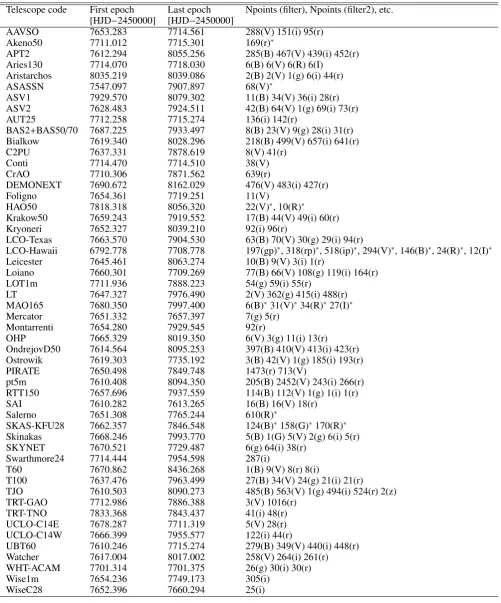
The follow-up observations started immediately after the an-nouncement of the alert (list of telescopes and their acronyms is provided in Tab.1), with the first data points taken on the night 9/10 Aug 2016 with the 0.6m Akdeniz Univ. UBT60 telescope in the TUBITAK National Observatory, Antalya, the SAI South-ern Station in Crimea, the pt5m telescope at the Roque de los Muchachos Observatory on La Palma (Hardy et al. 2015), the 0.8m Telescopi Joan Oro (TJO) at l’Observatori Astronomic del Montsec, and the 0.8m robotic APT2 telescope in Serra La Nave (Catania). The data showed a curious evolution and a gradual rise (0.1 mag/day) in the light curve without change in colour, atyp-ical for many known types of variable and cataclysmic variable stars. On the night 13/14 Aug 2016 (HJD0≡HJD-2450000.0∼
7614.5) the object reached a peak V=13.8 mag (B-V=1.6 mag, I=12.2 mag), as detected by ATP2 and TJO, which was followed by a sudden drop by about 2 magnitudes. Alerted by the unusual shape of the light curve we obtained spectra of Gaia16aye with the 1.22m Asiago telescope on 11 Aug and 2.0m Liverpool Tele-scope (LT, La Palma) on 12 Aug, which were consistent with a normal K8-M2 type star (Bakis et al. 2016). The stellar spectra along with the shape of the light curve implied that Gaia16aye was a binary microlensing event, which was detected byGaiaat its plateau between the two caustic crossings and we have ob-served the caustic exit with clear signatures of the finite source effects.
The continued follow-up after the first caustic exit revealed a very slow gradual rise in brightness (around 0.1 mag in a month). On 17 Sep 2016 it increased sharply by 2 mag (first spotted by the APT2 telescope), indicating the second caustic entry. The caustic crossing again showed a broad and long-lasting effect
19:40 19:40:20
19:40:40 19:41
19:41:20
+30:15
19:39:40 19:39:20 19:39
+30:10
+30:05
+30:00 DSS colored~1
1’ 33.97’ x 21.9’
N
E Powered by Aladin
20:00 00:00 22:00
02:00
+60:00 +65:00 +70:00
+55:00
18:00
VUL VUL CYG
CYG
AQL AQL
SCT SCT SER2 SER2 CEP
CEP
SGE SGE LYR
LYR
LAC LAC CAS
CAS
Mellinger color
15? 136.6? x 33.14?
N
E
Powered by Aladin
15o
1’ 5’’
Mellinger
DSS PS1
N
[image:5.595.57.545.67.346.2]E
Fig. 1.Location of Gaia16aye on the sky. Images from Mellinger and DSS were obtained using the Aladin tool.
of finite source size (flattened peak), lasting for nearly 48 hours between HJD0=7649.4 and 7651.4 and reaching about V=13.6 mag and I=12 mag. The caustic crossing was densely covered by the Liverpool Telescope and the 0.6m Ostrowik Observatory near Warsaw, Poland.
Following the second caustic entry, the object remained very bright (I∼12-14 mag) and was observed by multiple telescopes from around the globe, both photometrically and spectroscopi-cally. The complete list of telescopes and instruments involved in the follow-up observations of Gaia16aye is shown in Table 1 and their parameters are gathered in Table A.1 in the Ap-pendix. In total more than 25,000 photometric and more than 20 spectroscopic observations were taken over the period of about two years. In early November 2016 the brightness trend changed from falling to rising, as expected for binary events during the caustic crossing (Nesci 2016; Khamitov et al. 2016b). A simple preliminary model for the binary microlensing event predicted the caustic exit to occur around Nov 20.8 UT (HJD0=7713.3)
and the caustic crossing to last about 7 hours (Mroz et al. 2016). In order to catch and cover the caustic exit well, an intensive observing campaign was begun, involving also amateur astro-nomical associations (including the British Astroastro-nomical As-sociation and the German Haus der Astronomie) and school pupils. The observations were reported live also on Twitter (hashtag#Gaia16aye). A DDT observing time was allocated at the William Herschel Telescope (WHT/ACAM) and the Tele-scopio Nazionale Galileo (TNG/DOLORES) to provide low and high-resolution spectroscopy at times close to the peak. How-ever, the actual peak occurred about 20 hours later than expected, on 21 Nov 16 UT (7714.17), and was followed by TRT-GAO, Aries130, CrAO, AUT25, T60, T100, RTT150 (detection of the 4th caustic was reported in Khamitov et al. 2016a),
Montar-renti, Bialkow, Ostrowik, Krakow50, OndrejovD50, LT, pt5m, Salerno, UCLO, spanning the whole globe, which provided 24 hours coverage of the caustic exit. The sequence of spectroscopic observations before and at the very peak was taken with the IDS instrument on the Isaac Newton Telescope (INT). After the peak at 11.85 mag in I-band, the event’s brightness smoothly declined, as caught by Swarthmore24, DEMONEXT, and AAVSO. The first datapoint taken on the next night from India (Aries130 tele-scope) showed I=14.33 mag, indicating the complete exit from the caustic. The event then began rising very slowly again, with a rate of 1 mag over 4 months and exhibited a smooth peak on 05 May 2017 (HJD’=7878) reaching I=13.3 mag (G∼14 mag) (Wyrzykowski et al. 2017). After that, the light curve declined slowly and reached the pre-alert level in Nov 2017, at G=15.5 mag. We continued our photometric follow-up for another year to confirm there was no further re-brightening. Throughout the event, the All-Sky Automated Survey for SuperNovae (ASAS-SN) (Shappee et al. 2014; Kochanek et al. 2017a) was observing Gaia16aye serendipitously with a typical cadence of between 2 and 5 days. Its data covers various parts of the light curve of the event, including the part before theGaiaalert, where a smooth rise and the 1st caustic entry occurred.
2.1. Ground-based photometry calibrations
57500
57600
57700
57800
57900
58000
58100
MJD[days]
12
13
14
15
16
17
18
Brightness[mag]
I/i
R/r
V
g
B
Gaia ASAS-SN Loiano M.Chruslinska LCO F.Lewis Ondrejov M.Jelinek LT A.Gomboc UBT60 V.Bakis BAS 2 AUT25 V.Bakis Kryoneri A.Liakos TRT-TNO S.Awipan LOT1m H.Lee CrAO S.Nazarov
PIRATE U.Kolb Watcher
Bialkow P.Mikolajczyk T60 O.Erece Loiano G.Altavilla APT2 G.Leto AAVSO
Bialkow Z.Kolaczkowski Leicester K.Wiersema TRT-GAO S.Awipan Ostrowik M.Pawlak WiseC28 N.Hallakoun PIRATE M.Morrell
Loiano J.Klencki pt5m L.Hardy TJO U.Burgaz Loiano P.Iwanek Montarrenti Observatory ASV1 G.Damljanovic C2PU J.P.Rivet Mercator Geneva Group Skinakas P.Reig LCO D.Russell Krakow50 S.Kurowski UCLO-C14E S.Fossey Ostrowik K.Rybicki
D.Conti WHT K.Rybicki LCO K.Rybicki T100 H.Esenoglu ASV2 G.Damljanovic Loiano F.Cusano Aries130 G.Damljanovic Foligno R.Nesci SAI A.Zubareva LCO R.Street OHP M.Dennefeld RTT150 I.Khamitov
OHP M.Pawlak LOT1m C.Ngeow Wise1m G.Birenbaum T60 I.Khamitov UCLO-C14W S.Fossey Aristarchos K.Sokolovsky T60 Y.Kilic
BAS 50/70 Swarthmore24 E.Jensen Bialkow D.Mozdzierski DEMONEXT M.Penny SKYNET S.Zola
640
660
680
700
720
HJD-2457000
12
13
14
15
16
17
Brightness[mag]
714.0
714.4
714.8
HJD-2457000
12
13
14
15
16
[image:6.595.41.550.61.567.2]17
Fig. 2.Gaia, ASAS-SN and follow-up photometric observations of Gaia16aye. Each observatory/observer are marked with a different colour and marker explained in the legend. The figure shows only the follow-up data which were automatically calibrated using the Cambridge Photometric Calibration Server. The upper panel shows the entire event, while the bottom figures show zoom on the second pair of caustic crossings (left) and a detail of the fourth caustic crossing (right).
and Daophot (Stetson 1987). The lists of detected sources with their measured instrumental magnitudes were uploaded to the Cambridge Photometric Calibration Server (CPCS)3, designed and maintained by Sergey Koposov and Lukasz Wyrzykowski. The CPCS matches the field stars to a reference catalog, iden-tifies the target source and determines which filter was used for observations. This tool acted as a central repository for all the data, but primarily it standardised the data into a homogenous
3 http://gsaweb.ast.cam.ac.uk/followup
Onboard GRVS = 12.0 mag
845 850 855 860 865 870
Barycentric wavelength (nm) 0
10 20 30 40 50
[image:7.595.313.550.56.245.2]Flux (electrons per 0.025 nm wavelength bin)
Fig. 3.Medium-resolution spectrum of the Gaia16aye event obtained withGaia’s RVS at the brightest moment of the event as seen byGaia at the 4th caustic crossing. The lensed source’s CaII lines are clearly visible.
The list of all the ground-based photometric observations is summarised in Table 2 and the photometric observations are listed in Table C.1 available in the Appendix. The full table con-tains 23,730 entries and is available in the electronic version of the paper. Figure 2 shows all follow-up measurements collected for Gaia16aye over a period of about one and a half years.
2.2. Gaia data
Since October 2014 Gaia collected 27 observations before the alert on the 5th of August 2016. In total Gaia observed Gaia16aye 84 times as of November 2018. The G-band pho-tometric data points collected by Gaiaare listed in Table B.1. Photometric uncertainties are not provided for Gaiaalerts and for this event we assumed 0.01 mag (Gaia Collaboration et al. 2016), however, as shown later, these were scaled to about 0.015 mag by requiring the microlensing model’sχ2per degree of free-dom to be 1.0. Details of theGaiaphotometric system and its calibrations can be found in Evans et al. (2018).
Gaia’s on-board Radial Velocity Spectrometer (RVS), which operates at R∼11000, is collecting medium-resolution (R∼11,700) spectra over the wavelength range 845-872 nm cen-tred on in the Calcium II triplet region of objects brighter than V∼17 mag (Gaia Collaboration et al. 2016; Cropper et al. 2018). However, individual spectra for selected observations are made available already for brighterGaiaalerts using parts of the RVS data processing pipeline (Sartoretti et al. 2018). For Gaia16aye the RVS collected a spectrum on 2016-11-21 17:05:47 UT (HJD=2457714.21), see Figure 3, the moment caught byGaia at very high magnification, when Gaia16aye reached G=12.91 mag. The exposure time for the combined 3 RVS CCDs was 3×4.4 seconds.
2.3. Spectroscopy
Spectroscopic measurements of the event were obtained at vari-ous stages of its evolution. The list of spectroscopic observations is presented in Table 3. The very first set of spectra were taken with the Asiago 1.22 m telescope equipped with the
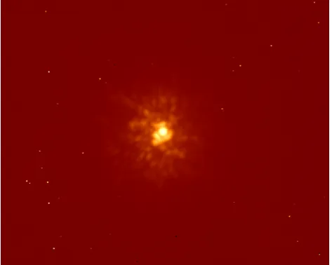
DU440A-Fig. 4.Keck Adaptive Optics image of Gaia16aye taken between the third and the fourth caustic crossing. The single star has a FWHM of about 52 mas. There are no other sources of light significantly con-tributing to the blending in the event.
8400 8500 8600 8700 8800
0.0
0.2
0.4
0.6
0.8
1.0
Nor
maliz
ed flux
Wavelength [A°]
INT spectrum (observed)
[image:7.595.54.282.64.235.2]synthetic spectrum Teff=3933 K, logg=2.2, [M/H]=0.08
Fig. 5.Spectrum of the source of the Gaia16aye event (blue) taken us-ing the 2.5-m INT/IDS in November 19, 2016 in comparison with a synthetic spectrum (red) calculated for the best fitted atmospheric pa-rameters. The plot shows the Ca II triplet region, 8400−8800 Å.
BU2 instrument, Asiago 1.82 m telescope with AFOSC and the SPRAT instrument on the 2 m Liverpool Telescope (LT), which showed no obvious features seen in outbursting Galactic vari-ables. Other spectra gathered by the 5 m P200 Palomar Hale Telescope as well as ACAM on the 4.2 m William Herschel Tele-scope (WHT), confirmed such behaviour. This, therefore, led us to conclude we are dealing with a microlensing event.
[image:7.595.308.549.340.562.2]re-gardless of whether the spectrum was recorded during amplifica-tion or in the baseline. This allows us to conclude that the spectra were dominated by the radiation from the source and contribu-tion from the lens was negligible.
Most of the spectra were obtained in low-resolution mode (R≤1000), and relatively poor weather conditions, which were useful for early classification of the transient as a microlensing event. More detailed analysis of the low-resolution spectra will be presented elsewhere (Zielinski M. et al., in prep.)
We have also obtained spectra of higher resolution (R ∼
6500) with the 2.5 m Isaac Newton Telescope (INT, La Palma, Canary Islands) during three consecutive nights on November 19−21, 2016. The INT spectra were obtained by using the In-termediate Dispersion Spectrograph (IDS, Cassegrain Focal Sta-tion, 235 mm focal length camera RED+2) with the grating set to R1200Y, and a dispersion of 0.53Å pixel−1with a slit width pro-jected onto the sky equal to 1.29800(see Tab. 3, spectrum INT 3–
5). The exposure time was 400 s for each spectrum centered at wavelength 8100Å.
The spectra were processed by the observers with their own pipelines or in a standard way using IRAF4 tasks and scripts. The reduction procedure consisted of the usual bias- and dark-subtraction, flat-field correction and wavelength calibration.
2.4. Swift observations
In order to rule out a possibility that Gaia16aye is some kind of cataclysmic variable star outburst, we requested X-ray and ultra-violet Swift observations. Swift observed Gaia16aye for 1.5ks on 2016-08-18. Swift/XRT detected no X-ray source at the position of the transient with an upper limit of 0.0007±0.0007 cts/s (a sin-gle background photon appeared in the source region during the exposure). Assuming a power law emission with a photon index of 2 and HI column density of 43.10×1020cm−2(corresponding to the total Galactic column density in this direction (Kalberla et al. 2005)), this translates to an unabsorbed 0.3-10 keV flux limit of 5.4×10⁻¹⁴ergs/cm2/s.
No ultraviolet source was detected by the UVOT instrument at the position of the transient and the upper limit at epoch HJD’=7618.86 was derived as >20.28 mag for UVM2-band (Vega system).
2.5. Keck Adaptive Optics imaging
The event was observed with Keck Adaptive Optics (AO) imag-ing on 8 Oct 2016 (HJD’=7669.7). Figure 4 shows the 10 arc-sec field-of-view obtained with the Keck AO instrument. The FWHM of the star is about 52 mas. The image shows a single object with no additional sources of light in its neighbourhood. This indicates no extra luminous components contributing to the observed light.
3. Spectroscopy of the source star
During a microlensing event the variation in the amplification changes the ratio of the flux coming from the source, while the blend or lens light remains at the same level. Therefore, the spec-troscopic data obtained at different amplifications can be used
4 IRAF is distributed by the National Optical Astronomy
Observato-ries, which are operated by the Association of Universities for Research in Astronomy, Inc., under cooperative agreement with the National Sci-ence Foundation.
to de-blend the light of the source from any additional constant components and to derive properties of the source.
In order to obtain the spectral type and stellar parameters of the Gaia16aye source, we used three spectra gathered by the 2.5 m INT. Based on these spectra we were able to determine the atmospheric parameters of the microlensing source. We used a dedicated spectral analysis framework – iSpec5which integrates several radiative transfer codes (Blanco-Cuaresma et al. 2014). In our case, the SPECTRUM code was used (Gray & Corbally 1994), together with well-known Kurucz model atmospheres (Kurucz 1993) and solar abundances of chemical elements taken from Asplund et al. (2009). The list of absorption lines with atomic data was taken from the VALD database (Kupka et al. 2011). We modelled synthetic spectra for the whole wavelength region between 7200–8800 Å. The spectrum which was synthe-sized to the observational data with the lowestχ2value consti-tutes the final fit generated for specific atmospheric parameters: effective temperature (Teff), surface gravity (log g) and metallic-ity ([M/H]). For simplification purposes, we adopted solar val-ues of micro– and macroturbulence velocities and also neglected stellar rotation. The resolution of the synthetic spectra was fixed as R = 10 000. We applied this methodology to all three INT spectra independently, and then, we averaged the results. The mean values for the parameters of the source in Gaia16aye were as follows: Teff = 3933 ±135 K, log g = 2.20±1.44 and [M/H]= 0.08±0.41 dex. Figure 5 presents the best fit of the synthetic to observational INT spectrum in the same spectral re-gion as covered by the RVS spectrum of Gaia16aye,i.e.,8400– 8800 Å (Ca II triplet), generated for averaged results of param-eters. These parameters imply that the microlensing source is a K5-type giant or a super-giant with solar metallicity. We discuss the estimate for the distance of the source in the next section, as first it is necessary to de-blend the light of the lens and the source which is possible from the microlensing model. We note that the asymmetry of the Gaia RVS lines is not visible in the same-resolution INT/IDS spectrum and we suspect the broaden-ing visible in the Gaia spectrum is a result of a stack of spectra from separate RVS CCDs.
4. Microlensing model
4.1. Data preparation
The data sets used in the modelling are listed in Table D.1 in the Appendix. Because of the complexity of the microlensing model, we had to restrict the number of data points used. We chose data sets that cover large parts of the light curve or im-portant features (such as caustics). Some of the available data sets were also disregarded, because they showed strong system-atic variations in residuals from the best-fit model, which are not supported by other data sets. We used observations collected in the CousinsI- or Sloani-band, because the signal-to-noise ra-tio in these filters is the largest. The only excepra-tions wereGaia (G-band filter) and ASAS-SN data (V-band), which cover large portions of the light curve, especially before the transient alert.
The calculation of microlensing magnifications (especially during caustic crossings) requires a lot of computational time. We thus binned the data to speed up the modelling. We usually used 1-day bins, except for caustic crossings (when brightness variations during one night are substantial), for which we used 0.5-hr or 1-hr bins.Gaiaand ASAS-SN data were not binned.
We rescaled the error bars, so thatχ2/dof ∼1 for each data set. The error bars were corrected using the formula σi,new =
p
(γσi)2+2. Coefficientsγand, for each data set, are shown
in Table 4. The final light curve is presented in Fig. 6.
4.2. Binary lens model
The simplest model describing a microlensing event caused by a binary system needs seven parameters: time of the closest ap-proach between the source and the center of mass of the lenst0, projected separation between source and barycenter of the lens at that timeu0(in Einstein radius units), the Einstein crossing time tE, mass ratio of the lens componentsq, projected separation be-tween two binary componentss, angle between the source-lens relative trajectory and the binary axisα, and the angular radius of the sourceρnormalized to the Einstein radius (Eq.1).
Such a simple model is insufficient to explain all features in the light curve. We therefore have to include additional pa-rameters that describe “second-order” effects: orbital motion of the Earth (“microlensing parallax”) and the orbital motion of the lens. The microlensing parallax πE = (πE,N, πE,E) is a vec-tor quantity:
πE=
πrel θE
µrel
µrel ,
where µrel is the relative lens-source proper motion (Gould 2000). It describes the shape of the relative lens-source trajec-tory (Fig. 7). The microlensing parallax can also be measured using simultaneous observations from two separated observato-ries, e.g., from the ground and a distant satellite (Refsdal 1966; Gould 1994). AsGaiais located at theL2Lagrange point (about 0.01 au from the Earth) and the Einstein radius projected onto the observer’s plane is au/πE ≈2.5 au, the magnification gradi-ent changes by less than the data precision throughout most of the light curve (see Fig. 8). Fortunately, twoGaiameasurements were collected near HJD0∼7714, when the space-parallax sig-nal is the strongest due to rapid change in magnification near the caustic. Therefore, we include the space-parallax andGaia observations in the final modelling.
The orbital motion of the lens, in the simplest scenario, can be approximated as linear changes of separations(t)=s0+s˙(t−
t0,kep) and angleα(t)=α0+α˙(t−t0,kep),t0,kepcan be any arbitrary
moment of time and is not a fit parameter (Albrow et al. 2000). That approximation, which works well for the majority of binary microlensing events, is insufficient in this case.
We have to describe the orbital motion of the lens using a full Keplerian approach (Skowron et al. 2011). This model is parameterised by the physical relative 3D position and velocity of the secondary component relative to the primary:
∆r=DlθE(s0,0,sz),∆v=DlθEs0(γx, γy, γz)
at timet0,kep. For a given angular radius of the source starθ∗and
source distanceDs, we can calculate the angular Einstein radius
θE = θ∗/ρ and distance to the lens Dl = au/(θEπE +au/Ds).
Subsequently, positions and velocities can be transformed to or-bital elements of the binary (semi-major axisa, orbital periodP, eccentricitye, inclinationi, longitude of the ascending nodeΩ, argument of periapsisω, and time of periastrontperi). These can be used to calculate the projected position of both components on the sky at any moment of time.
In all previous cases of binary events with the significant bi-nary motion, Keplerian orbital motion provides only a small im-provement relative to the linear approximation (Skowron et al. 2011; Shin et al. 2012). This is not the case here, because, as we
show below, the orbital period of the lens is similar to the du-ration of the event (e.g., Penny et al. 2011). Modelling of this event is an iterative process: for given microlensing parameters, we estimate the angular radius and distance to the source, we cal-culate best-fit microlensing parameters and repeat the procedure until all parameters converge.
The best-fit microlensing parameters are presented in Ta-ble 5. Uncertainties were calculated using the Markov chain Monte Carlo approach (Foreman-Mackey et al. 2013) and rep-resent 68% confidence intervals of marginalized posterior dis-tributions. We note that there exists another degenerate solution for the microlensing model, which differs only by signs of sz
andγz((sz, γz)→ −(sz, γz)). The second solution has the same
physical parameters (exceptΩ → π−Ωandω → ω−π) and differs by a sign of radial velocity. Thus, the degeneracy can be broken with additional radial velocity measurements of the lens (Skowron et al. 2011).
4.3. Source Star
Spectroscopic observations of the event indicate that the source is a K5-type giant or a super-giant. If the effective tempera-ture of the source were higher than 4250 K, TiO absorption fea-tures would be invisible. If the temperature were lower than 3800 K, these features would be stronger than those in the ob-served spectra. Indeed, spectral modelling indicates that the ef-fective temperature of the source is 3933±135 K. According to Houdashelt et al. (2000), the intrinsic Johnson-Cousins colours of a star of that spectral type and solar metallicity should be (V−R)0=0.83+−00..0312, (V−I)0=1.60+−00..0312and (V−K)0=3.64+−00..1137 (error bars correspond to the source of K4- and M0-type, respec-tively).
We use a model-independent regression to calculate ob-served colours of the source (we use observations collected in the Bialkow Observatory, which were calibrated to the standard system):V−R=0.99±0.01 andV−I=1.91±0.01. Thus, the colour excess isE(V−I) =0.31 andE(V−R)=0.16, consis-tent with the standard reddening law (Cardelli et al. 1989) and AV =0.62.
The best fitting microlensing model yields the amount of light coming from the magnified source, asVs = 16.61±0.02 andIs =14.70±0.02. TheV-band brightness of the source af-ter correcting for extinction is thereforeV0 = 15.99 mag. Sub-sequently, we use colour–surface brightness relations for giants from Adams et al. (2018) to estimate the angular radius of the source:θ∗ =9.2±0.7µas. As the linear radius of giants of that
spectral type is about 31±6R(Dyck et al. 1996), the source is
located about 15.7±3.0 kpc from the Sun, but the uncertainties are large. For the modelling we assumeDs = 15 kpc. We note
that the exact value of the distance has in practice a very small impact on the final models, becauseπsθEπE.
4.4. Physical parameters of the binary lens
The Gaia16aye microlensing model allows us to convert mi-crolensing quantities to physical properties of the lensing binary system. Finite source effects over the caustics enabled us to mea-sure the angular Einstein radius:
θE=
θ∗
ρ =3.04±0.24 mas and the relative lens-source proper motion:
µrel= θE tE
Because the microlensing parallax was precisely measured from the light curve (Table 5), we were able to measure the total mass of the lens:
M= θE
κπE =
0.93±0.09M
and its distance:
Dl=
au θEπE+au/Ds
=780±60 pc.
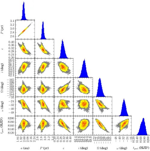
The orbital parameters of the lens were calculated using the pre-scriptions from Skowron et al. (2011) based on the full infor-mation about the relative 3D position and velocity of the sec-ondary star relative to the primary. All physical parameters of the lens are given in Table 6. Figure 9 shows the orbital param-eters and their confidence ranges as derived from the MCMC sampling of the microlensing model. Our microlensing model also allowed us to disentangle the flux from the source and the unmagnified blended flux (which we will show comes from the lens): Vblend = 17.98±0.02, Rblend = 17.05±0.02, and
Iblend=16.09±0.02 (Table 5).
5. Discussion
For Gaia16aye a massive follow-up campaign allowed us to col-lect a very detailed light curve and hence to cover the evolution of the event exhaustively. Photometric data were obtained over a period of more than 2 years by a network of observers scattered around the world. It should be emphasised that the vast major-ity of the observations were taken by enthusiastic individuals, including both professional astronomers and amateurs, who de-voted their telescope time to this task.
The case of Gaia16aye illustrates the power of coordi-nated long-term time-domain observations, leading to a scien-tific discovery. The field of microlensing particularly benefiting in the past from such follow-up observations, which resulted, for example, in the first microlensing planetary discoveries (e.g., Udalski et al. 2005; Beaulieu et al. 2006). This event also offered a dose of excitement with its multiple, rapid and often dramatic changes in brightness. Therefore it was also essential to use tools, which facilitated the observations and data processing. Of particular importance was the Cambridge Photometric Calibra-tion Server (CPCS, Zieli´nski et al. 2019), which performed the standardisation of the photometric observations collected by a large variety of different instruments. Moreover, the operation of the CPCS can be scripted, hence the observations could be auto-matically uploaded and processed without any human interven-tion. Such a solution helped track the evolution of the light curve especially at times when the event changed dramatically. The processed observations and photometric measurements were im-mediately available for everyone to view and appropriate actions were undertaken,e.g.,increase of the observing cadence when approaching the peak at the 4th caustic crossing. We note that for the part of the sky with the Gaia16aye event there were no archival catalogues available inIandRfilters. All the observa-tions carried in such filters were automatically adjusted by the CPCS to the nearest Sloaniandrbands. This does not affect the microlensing modelling, however, the standardised light curve iniandrfilters is systematically offset. On the other hand, the B−, g−andV−band observations processed by the CPCS are calibrated correctly to one percent level.
In the case of Gaia16aye the light curve contains multiple features, which allowed us to constrain the microlensing model uniquely, despite its complexity. Apart from the four caustic
crossings and a cusp approach, the microlensing model predicted also a smooth low-amplitude long-term bump about a year be-fore the first caustic crossing, at about HJD’=7350. Such a fea-ture was indeed found in theGaiadata, see Fig.6. The amplitude of this rise was about 0.1 mag, hence close to the level ofGaia’s photometric error bars and the signal was way too small to trig-ger an alert.
Additional confirmation of the correctness of the microlens-ing model comes from the detection of the microlensmicrolens-ing space-parallax effect, see Fig.8. The offset in the timing of the fourth caustic crossing as seen byGaiaand ground-based telescopes is due to the distance ofGaia1.5 million km away from Earth. The offset in time was 6.63h (i.e.,the caustic crossing by the source has happened first atGaia’s location) and the amplification dif-ference was -0.007 mag,i.e.,it was brighter atGaia. The model from ground-based data only predicted these offsets to within 3 minutes and 0.003 mag, respectively, therefore indicating our model is unique and robust.
From the microlensing light curve analysis one can derive an upper limit on the amount of light emitted by the lensing object or constraints on the dark nature of the lens can be obtained (e.g., Yee 2015; Wyrzykowski et al. 2016). We find that the masses of the lens components are 0.57±0.05Mand 0.36±0.03M
and that the lens is located about Dl = 780±60 pc from the
Sun. As theV-band absolute magnitudes of main-sequence stars of that masses are 8.62 and 11.14 (Pecaut & Mamajek 2013), respectively, the total brightness of the binary isV =17.97 and I =16.26, assuming conservativelyAV =0.1 towards the lens.
This is consistent with the brightness and colour of the blend
(Vblend =17.98 andIblend =16.09). The blended light therefore
comes from the lens, which is also consistent with the lack of any additional sources of light on the Keck AO image. This is an additional check that our model is correct.
The largest uncertainty in our lens mass determination comes from theθEparameter, which we derived from the finite source effects. Thanks to multiple caustic crossings, but particularly due to very detailed coverage of the fourth one with multiple obser-vatories, we were able to constrain the size of the source stellar disk in units of the Einstein radius (logρ) with less than one percent uncertainty. However, in order to deriveθE, we relied on the colour-angular size relation and theoretical predictions for the de-reddened colour of the source based on its spectral type. These may have introduced systematic errors to the angular size and hence to the lens mass measurement. We also note that the amount of the extinction derived based on our photometry (AV =0.62 mag) is significantly smaller than that measured by
Schlafly & Finkbeiner (2011) in this direction (AV =1.6 mag).
This and the uncertainty in the physical size of giant stars, af-fects the estimate of the source distance, however, since the lens is very nearby at less than 1 kpc, the source distance does not affect the overall result of this study.
Nevertheless, an independent measurement of the Einstein radius, and thus the final confirmation of the nature of the lens in Gaia16aye, can be obtained in the near future fromGaia astro-metric time-domain data. Using our photometry-based model, we computed the positions and amplifications of the images throughout the evolution of the event. Figure 10 shows the ex-pected position of the combined light of all the images shown in the frame of the centre of mass of the binary and in units of the Einstein radius. The figure shows only the centroid motion due to microlensing relative to the unlensed position of the source. The moments ofGaiaobservations are marked with black dots. Since θE =3.04±0.24 mas, the expected amplitude of the astrometric
as-11.6
12.0
12.4
12.8
13.2
13.6
14.0
14.4
14.8
Magnitude
Gaia BialkowI
APT2I
LTi
DEMONEXTI
SwarthmoreI
UBT60I
ASAS-SNV
7200 7300 7400 7500 7600 7700 7800 7900 8000
HJD - 2450000 −0.20
−0.15
−0.10
−0.05
0.00
0.05
0.10
0.15
[image:11.595.43.547.61.362.2]Residual
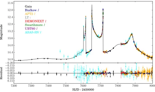
Fig. 6.Light curve of the microlensing event Gaia16aye, showing only the data used in the microlensing model. All measurements are transformed to the LTi-band magnitude scale.
trometric time-series asGaiais expected to have the error-bars in the along-scan direction of order of 0.1 mas (Rybicki et al. 2018). The estimate ofθEfromGaiawill be free of our assump-tions about the intrinsic colours of the source and the interstellar extinction. The actual Gaia astrometry will include also the ef-fects of parallax and proper motion of the source as well as the blended light from both components of the binary lens. The con-tribution of the lens brightness to the total light is about 25%, therefore the astrometric data might also be affected by the or-bital motion of the binary. It is worth emphasising that without the microlensing model presented above, obtained from photo-metric Gaia and follow-up data only, the interpretation of the Gaia astrometry will not be possible due to the large complexity of centroid motion.
Radial Velocity measurements of nearby binary lenses offer an additional way for post-event verification of the orbital pa-rameters inferred from the microlensing model. So far, such an attempt was successfully achieved only in the case of OGLE-2009-BLG-020, a binary lens event with a clear orbital mo-tion effect (Skowron et al. 2011). Follow-up observations from Keck and Magellan telescopes measured the radial velocity (RV) of the binary to agree with the one predicted based on the microlensing event full binary lens orbit solution (Yee et al. 2016). The binary system presented in this work (to be de-noted as Gaia16aye-L, with its components Gaia16aye-La and Gaia16aye-Lb) is nearby (780±60 pc) and fairly bright (I∼16.5 mag without the source star), hence such observations are ob-tainable. The expected amplitude of the radial velocity curve of the primary is about K≈7.6 km/s. We strongly encourage for such observations to be carried out in order to verify the binary solution found in microlensing.
Yet another possibility to verify the model might come from Adaptive Optics or other high resolution imaging techniques (e.g., Scott 2019) in couple of years when the source and the lens separate (e.g., Jung et al. 2018). With the relative proper motion of 10.1±0.8 mas yr−1, the binary lens should become visible at a separation of about 50 mas already in 2021.
6. Conclusions
We analysed the long-lasting event Gaia16aye, which exhibited four caustic crossings and a cusp approach, as well as space-parallax between the Earth and theGaiaspacecraft.
The very well-sampled light curve allowed us to determine the masses of the binary system (0.57±0.05 Mand 0.36±0.03
M) and all its orbital components. We derived the period
(2.88±0.05 years) and semi-major axis (1.98±0.03 au), as well as the eccentricity of the orbit (0.30±0.03). Gaia16aye is one of only a few microlensing binary systems with the full orbital so-lution, which offer an opportunity for confirmation of the binary parameters with the radial velocity measurements and high res-olution imaging after couple of years. This event will also be de-tectable as an astrometric microlensing event in the forthcoming Gaiaastrometric time-series data.
−0.6 −0.4 −0.2 0.0 0.2 0.4 0.6 0.8 1.0
x(θE)
−0.8 −0.6 −0.4 −0.2 0.0 0.2 0.4 0.6 0.8 y ( θE ) N E
HJD0=7602
HJD0=7614
HJD0=7649
HJD0=7714 HJD0=7878
0.15 0.20 0.25
0.20 0.25
Earth
[image:12.595.44.278.58.293.2]Gaia
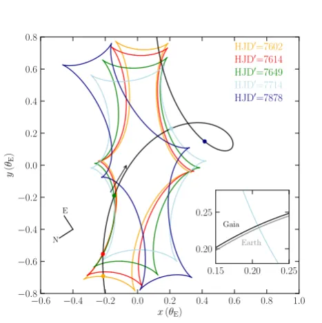
Fig. 7.The caustic curves corresponding to the best-fitting model of Gaia16aye. The lens-source relative trajectory is shown by a black curve. The barycenter of the lens is at (0,0) and the lens components are located along thexaxis at timet0,kep=7675. Caustics are plotted at
the times of caustic crossings with the large points marked with respec-tive colours. The inset shows a zoom on the trajectory of the Earth and Gaia at the moment of the caustic crossing around HJD0∼
7714.
automated analysis of the follow-up data and light curve gener-ation will soon become new standards in transient time-domain astronomy. The case of Gaia16aye shows that microlensing can be a useful tool for studying also binary systems where the lens-ing is caused by dark objects. A detection of a microlenslens-ing bi-nary system composed of black holes and neutron stars would provide information about that elusive population of remnants complementary to other studies.
Acknowledgements. This work relies on the results from the European Space Agency (ESA) space missionGaia.Gaiadata are being processed by theGaia
Data Processing and Analysis Consortium (DPAC). Funding for the DPAC is provided by national institutions, in particular the institutions participating in the Gaia Multi-Lateral Agreement (MLA). The Gaiamission website is https://www.cosmos.esa.int/gaia. In particular we acknowledgeGaia Photomet-ric Science Alerts Team, website http://gsaweb.ast.cam.ac.uk/alerts. We thank the members of the OGLE team for discussions and support. We also would like to thank the Polish Children Fund (KFnRD) for support of an internship of their pupils in Ostrowik Observatory of the Warsaw University, during which some of the data were collected, in particular we thank: Robert Nowicki, Michał Por ˛ebski and Karol Niczyj. The work presented here has been supported by the following grants from the Polish National Science Centre (NCN): HARMONIA NCN grant 2015/18/M/ST9/00544, OPUS NCN grant 2015/17/B/ST9/03167, DAINA NCN grant 2017/27/L/ST9/03221, as well as European Commission’s FP7 and H2020 OPTICON grants (312430 and 730890), Polish Ministry of Higher Education support for OPTICON FP7, 3040/7.PR/2014/2, MNiSW grant DIR/WK/2018/12. PMr and JS acknowledge support from MAESTRO NCN grant 2014/14/A/ST9/00121 to Andrzej Udalski. We would like to thank the following members of the AAVSO for their amazing work with collecting vast amounts of data: Teofilo Arranz, James Boardman, Stephen Brincat, Ge-offChaplin, Emery Erdelyi, Rafael Farfan, William Goff, Franklin Guenther, Kevin Hills, Jens Jacobsen, Raymond Kneip, David Lane, Fernando Limon Martinez, Gianpiero Locatelli, Andrea Mantero, Attila Madai, Peter Meadows, Otmar Nickel, Arto Oksanen, Luis Perez, Roger Pieri, Ulisse Quadri, Diego Rodriguez Perez, Frank Schorr, George Sjoberg, Andras Timar, Ray Tomlin, Tonny Vanmunster, Klaus Wenzel, Thomas Wikander. We also thank the am-ateur observers from around the world, in particular, Pietro Capuozzo, Leone Trascianelli, Igor Zharkov from Ardingly College and Angelo Tomassini, Karl-Ludwig Bath. We also thank Roger Pickard from the British Astronomical
11
.
6
12
.
0
12
.
4
12
.
8
13
.
2
13
.
6
14
.
0
14
.
4
14
.
8
Magnitude
Gaia
ground-based follow-up
7600
7605
7610
7615
7620
HJD - 2450000
−
0
.
20
−
0
.
15
−
0
.
10
−
0
.
05
0
.
00
0
.
05
0
.
10
0
.
15
Residual
7649
7651
HJD - 2450000
7713
7715
[image:13.595.74.489.94.399.2]HJD - 2450000
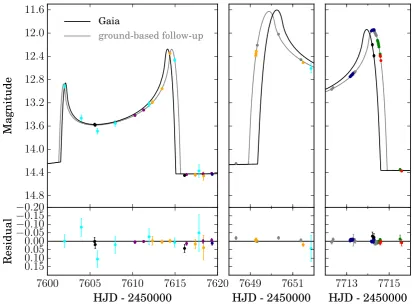
Fig. 8.Space-based parallax in Gaia16aye. AsGaiais separated by 0.01 au from the Earth, theGaialight curve (black) differs slightly from Earth-based observations (grey curve). Space-parallax can be measured thanks to two fortuitousGaiadata points collected near HJD0∼7714. All measurements are transformed to the LTi-band magnitude scale.
and no. 176021 ”Visible and invisible matter in nearby galaxies: theory and ob-servations” supported by the Ministry of Education, Science and Technological Development of the Republic of Serbia. YT acknowledges the support of DFG priority program SPP 1992 ”Exploring the diversity of Extrasolar Planets” (WA 1074/11-1). This work of PMi, DM and ZK was supported by the NCN grant no. 2016/21/B/ST9/01126. ARM acknowledges support from the MINECO Ramón y Cajal programme RYJ-2016-20254 and grant AYA2017-86274-P and from the AGAUR grant SGR-661/2017. The work by C.R. was supported by an appoint-ment to the NASA Postdoctoral Program at the Goddard Space Flight Center, administered by USRA through a contract with NASA. The Faulkes Telescope Project is an education partner of Las Cumbres Observatory (LCO). The Faulkes Telescopes are maintained and operated by LCO. This research was made possi-ble through the use of the AAVSO Photometric All-Sky Survey (APASS), funded by the Robert Martin Ayers Sciences Fund and NSF AST-1412587. The Pan-STARRS1 Surveys (PS1) and the PS1 public science archive have been made possible through contributions by the Institute for Astronomy, the University of Hawaii, the Pan-STARRS Project Office, the Max-Planck Society and its partic-ipating institutes, the Max Planck Institute for Astronomy, Heidelberg and the Max Planck Institute for Extraterrestrial Physics, Garching, The Johns Hopkins University, Durham University, the University of Edinburgh, the Queen’s Univer-sity Belfast, the Harvard-Smithsonian Center for Astrophysics, the Las Cumbres Observatory Global Telescope Network Incorporated, the National Central Uni-versity of Taiwan, the Space Telescope Science Institute, the National Aeronau-tics and Space Administration under Grant No. NNX08AR22G issued through the Planetary Science Division of the NASA Science Mission Directorate, the National Science Foundation Grant No. AST-1238877, the University of Mary-land, Eotvos Lorand University (ELTE), the Los Alamos National Laboratory, and the Gordon and Betty Moore Foundation. Some of the data presented herein were obtained at the W. M. Keck Observatory, which is operated as a scientific partnership among the California Institute of Technology, the University of Cali-fornia and the National Aeronautics and Space Administration. The Observatory was made possible by the generous financial support of the W. M. Keck Founda-tion.
References
Abbott, B. P., Abbott, R., Abbott, T. D., et al. 2016, Physical Review X, 6, 041015
Abbott, B. P., Abbott, R., Abbott, T. D., et al. 2017, Physical Review Letters, 118, 221101
Adams, A. D., Boyajian, T. S., & von Braun, K. 2018, MNRAS, 473, 3608 Albrow, M., Beaulieu, J.-P., Birch, P., et al. 1998, ApJ, 509, 687
Albrow, M. D., Beaulieu, J.-P., Caldwell, J. A. R., et al. 2000, ApJ, 534, 894 Alcock, C., Allsman, R. A., Alves, D., et al. 1997, ApJ, 479, 119
An, J. H. & Gould, A. 2001, ApJ, 563, L111
Asplund, M., Grevesse, N., Sauval, A. J., & Scott, P. 2009, ARA&A, 47, 481 Bachelet, E., Beaulieu, J.-P., Boisse, I., Santerne, A., & Street, R. A. 2018, ApJ,
865, 162
Bakis, V., Burgaz, U., Butterley, T., et al. 2016, The Astronomer’s Telegram, 9376
Beaulieu, J.-P., Bennett, D. P., Fouqué, P., et al. 2006, Nature, 439, 437 Belczynski, K., Holz, D. E., Bulik, T., & O’Shaughnessy, R. 2016, Nature, 534,
512
Belokurov, V. A. & Evans, N. W. 2002, MNRAS, 331, 649 Bennett, D. P., Rhie, S. H., Udalski, A., et al. 2016, AJ, 152, 125 Bertin, E. & Arnouts, S. 1996, A&AS, 117, 393
Bird, S., Cholis, I., Muñoz, J. B., et al. 2016, Physical Review Letters, 116, 201301
Blanco-Cuaresma, S., Soubiran, C., Jofré, P., & Heiter, U. 2014, A&A, 566, A98 Boisse, I., Santerne, A., Beaulieu, J.-P., et al. 2015, A&A, 582, L11
Bond, I. A., Udalski, A., Jaroszy´nski, M., et al. 2004, ApJ, 606, L155 Bozza, V. 2001, A&A, 374, 13
Brown, T. M., Baliber, N., Bianco, F. B., et al. 2013, Publications of the Astro-nomical Society of the Pacific, 125, 1031
Calchi Novati, S. & Scarpetta, G. 2016, ApJ, 824, 109
Fig. 9.Orbital elements of Gaia16aye. Panels show 2D and 1D projections of posterior distributions in the space of Kepler parameters. Red, orange and yellow points mark 1σ, 2σ, and 3σconfidence regions, respectively.
Dominik, M. & Sahu, K. C. 2000, ApJ, 534, 213
Dong, S., Mérand, A., Delplancke-Ströbele, F., et al. 2019, ApJ, 871, 70 Dyck, H. M., Benson, J. A., van Belle, G. T., & Ridgway, S. T. 1996, AJ, 111,
1705
Evans, D. W., Riello, M., De Angeli, F., et al. 2018, A&A, 616, A4
Foreman-Mackey, D., Hogg, D. W., Lang, D., & Goodman, J. 2013, PASP, 125, 306
French, J., Hanlon, L., McBreen, B., et al. 2004, in American Institute of Physics Conference Series, Vol. 727, Gamma-Ray Bursts: 30 Years of Discovery, ed. E. Fenimore & M. Galassi, 741–744
Fukui, A., Abe, F., Ayani, K., et al. 2007, ApJ, 670, 423
Fukui, A., Suzuki, D., Koshimoto, N., et al. 2019, arXiv e-prints, arXiv:1909.11802
Gaia Collaboration, Brown, A. G. A., Vallenari, A., et al. 2018, A&A, 616, A1 Gaia Collaboration, Prusti, T., de Bruijne, J. H. J., et al. 2016, A&A, 595, A1
Gaudi, B. S., Patterson, J., Spiegel, D. S., et al. 2008, The Astrophysical Journal, 677, 1268
Goudis, C., Hantzios, P., Boumis, P., et al. 2010, in Astronomical Society of the Pacific Conference Series, Vol. 424, 9th International Conference of the Hel-lenic Astronomical Society, ed. K. Tsinganos, D. Hatzidimitriou, & T. Mat-sakos, 422
Gould, A. 1992, ApJ, 392, 442 Gould, A. 1994, ApJ, 421, L75 Gould, A. 2000, ApJ, 542, 785
Gould, A. & Loeb, A. 1992, ApJ, 396, 104
Gould, A., Udalski, A., Monard, B., et al. 2009, ApJ, 698, L147 Gray, R. O. & Corbally, C. J. 1994, AJ, 107, 742
Hamadache, C., Le Guillou, L., Tisserand, P., et al. 2006, A&A, 454, 185 Han, C. 2008, ApJ, 681, 806
−0.8 −0.6 −0.4 −0.2 0.0 0.2 0.4 0.6 0.8 1.0
δθx(θE)
−0.8 −0.6 −0.4 −0.2 0.0 0.2 0.4 0.6 0.8 1.0 δθy ( θE )
6500<HJD0<7602 7602<HJD0<7614
7614<HJD0<7649
7649<HJD0<7713
7714<HJD0<8200
Gaiatransits
[image:15.595.44.279.60.292.2]N E
Fig. 10.As the source star moves across the caustics, new images of the source can be created while others may disappear, resulting in the changes of the image centroid. Colour curves show the path of the cen-troid of source images relative to the unlensed position of the source (additional light from components of the lens is not included). Moments ofGaiatransits are marked with black points. The coordinate system is the same as in Fig. 7. The shifts are scaled to the angular Einstein radius of the system (θE =3.04±0.24 mas). Analysis of theGaiaastrometric
measurements will provide an independent estimate ofθE.
Hodgkin, S. T., Wyrzykowski, L., Blagorodnova, N., & Koposov, S. 2013, Philosophical Transactions of the Royal Society of London Series A, 371, 20120239
Hogg, D. W., Blanton, M., Lang, D., Mierle, K., & Roweis, S. 2008, in As-tronomical Society of the Pacific Conference Series, Vol. 394, AsAs-tronomical Data Analysis Software and Systems XVII, ed. R. W. Argyle, P. S. Bunclark, & J. R. Lewis, 27
Houdashelt, M. L., Bell, R. A., Sweigart, A. V., & Wing, R. F. 2000, AJ, 119, 1424
Jaroszynski, M., Udalski, A., Kubiak, M., et al. 2004, Acta Astron., 54, 103 Jung, Y. K., Han, C., Udalski, A., et al. 2018, ApJ, 863, 22
Kains, N., Calamida, A., Sahu, K. C., et al. 2017, ApJ, 843, 145
Kalberla, P. M. W., Burton, W. B., Hartmann, D., et al. 2005, A&A, 440, 775 Khamitov, I., Bikmaev, I., Burenin, R., et al. 2016a, The Astronomer’s Telegram,
9780
Khamitov, I., Bikmaev, I., Burenin, R., et al. 2016b, The Astronomer’s Telegram, 9753
Kim, S.-L., Lee, C.-U., Park, B.-G., et al. 2016, Journal of Korean Astronomical Society, 49, 37
Kiraga, M. & Paczynski, B. 1994, ApJ, 430, L101
Kochanek, C. S., Shappee, B. J., Stanek, K. Z., et al. 2017a, PASP, 129, 104502 Kochanek, C. S., Shappee, B. J., Stanek, K. Z., et al. 2017b, PASP, 129, 104502 Kolb, U., Brodeur, M., Braithwaite, N., & Minocha, S. 2018, Robotic Telescope,
Student Research and Education Proceedings, 1, 127
Kozłowski, S., Wo´zniak, P. R., Mao, S., & Wood, A. 2007, ApJ, 671, 420 Kupka, F., Dubernet, M.-L., & VAMDC Collaboration. 2011, Baltic Astronomy,
20, 503
Kurucz, R. 1993, ATLAS9 Stellar Atmosphere Programs and 2 km/s grid. Ku-rucz CD-ROM No. 13. Cambridge, Mass.: Smithsonian Astrophysical Ob-servatory, 1993., 13
Lang, D., Hogg, D. W., Mierle, K., Blanton, M., & Roweis, S. 2010, AJ, 139, 1782
Lu, J. R., Sinukoff, E., Ofek, E. O., Udalski, A., & Kozlowski, S. 2016, ApJ, 830, 41
Mróz, P., Udalski, A., Skowron, J., et al. 2017, Nature, 548, 183
Mroz, P., Wyrzykowski, L., Rybicki, K., et al. 2016, The Astronomer’s Telegram, 9770
Nesci, R. 2016, The Astronomer’s Telegram, 9533
Nucita, A. A., Licchelli, D., De Paolis, F., et al. 2018, Monthly Notices of the Royal Astronomical Society, 476, 2962
Paczy´nski, B. 1971, Annual Review of Astronomy and Astrophysics, 9, 183 Paczynski, B. 1996, ARA&A, 34, 419
Pecaut, M. J. & Mamajek, E. E. 2013, ApJS, 208, 9
Penny, M. T., Kerins, E., & Mao, S. 2011, MNRAS, 417, 2216
Pietrzy´nski, G., Thompson, I. B., Gieren, W., et al. 2010, Nature, 468, 542 Poleski, R., Skowron, J., Udalski, A., et al. 2014, The Astrophysical Journal,
795, 42
Poleski, R., Zhu, W., Christie, G. W., et al. 2016, ApJ, 823, 63
Popowski, P., Alcock, C., Allsman, R. A., et al. 2001, in Astronomical Society of the Pacific Conference Series, Vol. 239, Microlensing 2000: A New Era of Microlensing Astrophysics, ed. J. W. Menzies & P. D. Sackett, 244 Popper, D. M. 1967, Annual Review of Astronomy and Astrophysics, 5, 85 Rahal, Y. R., Afonso, C., Albert, J. N., et al. 2009, Astronomy and Astrophysics,
500, 1027
Rattenbury, N. J. 2009, MNRAS, 392, 439 Refsdal, S. 1966, MNRAS, 134, 315
Rybicki, K. A., Wyrzykowski, Ł., Klencki, J., et al. 2018, MNRAS, 476, 2013 Sahu, K. C., Anderson, J., Casertano, S., et al. 2017, in American Astronomical
Society Meeting Abstracts, Vol. 230, American Astronomical Society Meet-ing Abstracts #230, 315.13
Sartoretti, P., Katz, D., Cropper, M., et al. 2018, A&A, 616, A6 Schlafly, E. F. & Finkbeiner, D. P. 2011, ApJ, 737, 103
Scott, N. J. 2019, in AAS/Division for Extreme Solar Systems Abstracts, Vol. 51, AAS/Division for Extreme Solar Systems Abstracts, 330.15
Shappee, B. J., Prieto, J. L., Grupe, D., et al. 2014, ApJ, 788, 48 Shin, I.-G., Han, C., Choi, J.-Y., et al. 2012, ApJ, 755, 91 Shvartzvald, Y., Li, Z., Udalski, A., et al. 2016, ApJ, 831, 183 Shvartzvald, Y., Udalski, A., Gould, A., et al. 2015, ApJ, 814, 111 Skowron, J., Jaroszynski, M., Udalski, A., et al. 2007, Acta Astron., 57, 281 Skowron, J., Udalski, A., Gould, A., et al. 2011, ApJ, 738, 87
Skowron, J., Wyrzykowski, Ł., Mao, S., & Jaroszy´nski, M. 2009, MNRAS, 393, 999
Sokolovsky, K., Korotkiy, S., & Lebedev, A. 2014, in Astronomical Society of the Pacific Conference Series, Vol. 490, Stellar Novae: Past and Future Decades, ed. P. A. Woudt & V. A. R. M. Ribeiro, 395
Steele, I. A., Smith, R. J., Rees, P. C., et al. 2004, in Proc. SPIE, Vol. 5489, Ground-based Telescopes, ed. J. M. Oschmann, Jr., 679–692
Stetson, P. B. 1987, PASP, 99, 191
Sumi, T., Bennett, D. P., Bond, I. A., et al. 2013, ApJ, 778, 150 Udalski, A., Han, C., Bozza, V., et al. 2018, ApJ, 853, 70
Udalski, A., Jaroszy´nski, M., Paczy´nski, B., et al. 2005, ApJ, 628, L109 Udalski, A., Szymanski, M., Mao, S., et al. 1994a, ApJ, 436, L103
Udalski, A., Szymanski, M., Stanek, K. Z., et al. 1994b, Acta Astron., 44, 165 Udalski, A., Szyma´nski, M. K., & Szyma´nski, G. 2015a, Acta Astron., 65, 1 Udalski, A., Yee, J. C., Gould, A., et al. 2015b, ApJ, 799, 237
Udalski, A., Zebrun, K., Szymanski, M., et al. 2000, Acta Astron., 50, 1 Villanueva, Steven, J., Gaudi, B. S., Pogge, R. W., et al. 2018, Publications of
the Astronomical Society of the Pacific, 130, 015001 Witt, H. J. & Mao, S. 1995, ApJ, 447, L105
Wozniak, P. R., Udalski, A., Szymanski, M., et al. 2001, Acta Astron., 51, 175 Wyrzykowski, Ł. & Hodgkin, S. 2012, in IAU Symposium, Vol. 285, New
Hori-zons in Time Domain Astronomy, ed. E. Griffin, R. Hanisch, & R. Seaman, 425–428
Wyrzykowski, L., Hodgkin, S., & Blagorodnova, N. 2014, in Gaia-FUN-SSO-3, 31
Wyrzykowski, Ł., Hodgkin, S., Blogorodnova, N., Koposov, S., & Burgon, R. 2012, in 2nd Gaia Follow-up Network for Solar System Objects, 21 Wyrzykowski, Ł., Kostrzewa-Rutkowska, Z., Skowron, J., et al. 2016, MNRAS,
458, 3012
Wyrzykowski, L., Mroz, P., Rybicki, K., et al. 2017, The Astronomer’s Telegram, 10341
Wyrzykowski, Ł., Rynkiewicz, A. E., Skowron, J., et al. 2015, ApJS, 216, 12 Xilouris, E. M., Bonanos, A. Z., Bellas-Velidis, I., et al. 2018, A&A, 619, A141 Yee, J. C. 2015, ApJ, 814, L11
Yee, J. C., Johnson, J. A., Skowron, J., et al. 2016, ApJ, 821, 121 Yee, J. C., Udalski, A., Calchi Novati, S., et al. 2015, ApJ, 802, 76
Yock, P. C. M. 1998, in Frontiers Science Series 23: Black Holes and High En-ergy Astrophysics, ed. H. Sato & N. Sugiyama, 375
Yoo, J., DePoy, D. L., Gal-Yam, A., et al. 2004, ApJ, 603, 139 Zhu, W., Calchi Novati, S., Gould, A., et al. 2016, ApJ, 825, 60
Zieli´nski, P., Wyrzykowski, Ł., Rybicki, K., et al. 2019, Contributions of the Astronomical Observatory Skalnate Pleso, 49, 125