Euler principal component analysis

DOI 10.1007/s11263-012-0558-z

Euler Principal Component Analysis

Stephan Liwicki·Georgios Tzimiropoulos· Stefanos Zafeiriou·Maja Pantic

Received: 5 December 2011 / Accepted: 8 August 2012 © Springer Science+Business Media, LLC 2012

Abstract Principal Component Analysis (PCA) is perhaps the most prominent learning tool for dimensionality reduc-tion in pattern recognireduc-tion and computer vision. However, the2-norm employed by standard PCA is not robust to out-liers. In this paper, we propose a kernel PCA method for fast and robust PCA, which we call Euler-PCA (e-PCA). In particular, our algorithm utilizes a robust dissimilarity measure based on the Euler representation of complex num-bers. We show that Euler-PCA retains PCA’s desirable prop-erties while suppressing outliers. Moreover, we formulate Euler-PCA in an incremental learning framework which al-lows for efficient computation. In our experiments we apply Euler-PCA to three different computer vision applications for which our method performs comparably with other state-of-the-art approaches.

Electronic supplementary material The online version of this article

(doi:10.1007/s11263-012-0558-z) contains supplementary material, which is available to authorized users.

S. Liwicki (

e-mail:[email protected] S. Zafeiriou

e-mail:[email protected] M. Pantic

e-mail:[email protected] G. Tzimiropoulos

School of Computer Science, University of Lincoln, Brayford Pool, Lincoln, LN6 7TS, UK

e-mail:[email protected] M. Pantic

Faculty of Electrical Engineering, Mathematics and Computer Science, University of Twente, Enschede, The Netherlands

Keywords Euler PCA·Robust subspace·Online learning·Tracking·Background modeling

1 Introduction

In pattern recognition, Principal Component Analysis (PCA) is perhaps the most classical tool for dimensionality reduc-tion and feature extracreduc-tion. It is widely utilized in a great va-riety of disciplines, including agriculture, biology and eco-nomics (Jolliffe2002). Researchers in computer vision em-ploy PCA for face recognition (Turk and Pentland1991), object tracking (Ross et al.2008), background modeling (Li 2004) and many other applications (Jolliffe 2002). It has been primarily used for efficient dimensionality reduction such that most of the variance of the original high dimen-sional data is preserved.

Given a population ofnsamples X= [x1· · ·xn] ∈Rp×n in ap-dimensional vector space,1standard PCA finds a set ofm≤p(usually,mp) orthonormal basis functions B= [b1· · ·bm] ∈Rp×mby minimizing the error functionϕwith respect to B

B=arg min ˇ

B

ϕ(B)ˇ =arg min ˇ

B

_{X− ˇB}BˇTX2_F, (1)

where.F denotes the Frobenius norm. It can be shown (Jolliffe2002) that the solution is given by the eigenvectors corresponding to the mlargest eigenvalues obtained from the eigendecomposition of the covariance matrix S=XXT (or the Singular Value Decomposition (SVD) of X).

The2-norm in (1) is optimal for the case of independent and identically distributed (i.i.d.) Gaussian noise but not ro-bust to outliers (de la Torre and Black2003; He et al.2011;

Kwak2008). Recent methods attempt to mitigate this sensi-tivity by adopting different error functions (He et al.2011; Ding et al.2006; Kwak2008; Ke and Kanade2003,2005; Candés et al.2009; de la Torre and Black2003) which, how-ever, often result in loss of efficiency. A reformulation of PCA in the context of M-Estimation is introduced in de la Torre and Black (2003). In Candés et al. (2009), PCA is rep-resented as an optimization problem which finds a low di-mensional linear subspace and a sparse matrix which repre-sents the outliers. Other approaches in the literature use vari-ants of the1-norm which are, in general, more robust than the2-norm (Ke and Kanade2003,2005; Ding et al.2006; Kwak2008; Mei and Ling 2009). More specifically, in Ke and Kanade (2003) and Ke and Kanade (2005) the optimiza-tion problem is considered with the following error funcoptimiza-tion

ϕ(B)=X−BBTX₁. (2)

The proposed 1-norm minimization is based on (i) the weighted median algorithm and (ii) convex quadratic pro-gramming, respectively. While this approach reduces the ef-fect of outliers, the optimization of (2) is computationally expensive. Moreover, both methods are not invariant to rota-tions, which is an important property of learning algorithms (Ding et al.2006).

The rotationally invariant R1-PCA (Ding et al.2006) is also based on the1-norm PCA

ϕ(B)= n

j=1

p

c=1

xj(c)− m

l=1 bl(c)

p

r=1

bl(r)xj(r)

2

, (3)

where xj(c)is thecth element of xj. PCA-L1 (Kwak2008) estimates the optimum of (2) with a componentwise greedy search for

B=arg max ˇ

B

BˇTX₁. (4)

Both methods allow for faster convergence towards the so-lution. Furthermore, both are rotational invariant. Most re-cently, Half-Quadratic PCA (HQ-PCA) is introduced in He et al. (2011). Here, the authors propose a rotational invari-ant and robust PCA using the maximum correntropy crite-rion (MCC) (Liu et al.2007). Correntropy is closely related to M-Estimators while the objective function is efficiently optimized by the half-quadratic optimization technique. In contrast to the proposed method, incremental implementa-tions of the above methods are unknown and therefore they are computationally expensive for large training sets and un-suitable for online learning.

Some of the problems often associated with robustness in PCA might be solved by more flexible modeling using Kernel PCA (KPCA) and more specifically by de-noising in feature spaces via the use of pre-images (Kwok and Tsang 2004; Mika et al. 1999; Honeine and Richard2011). The problem of sample de-noising in feature space is formulated

as follows. Letk(., .)be a positive definite function, the so-called kernel, and an implicit mappingφ, associated with the kernel, from the input space to a (possible) infinite dimen-sional Hilbert space. KPCA learns a linear subspace B in this high dimensional space. Then, a sample x is de-noised by solving the following optimization problem (Mika et al. 1999)

˜

x=arg min ˇ

x

φ (x)ˇ −BBTφ (x)2_F. (5)

Put in simple terms, the above optimization problem aims to find a samplex in input space such that its mapping in the˜ feature space φ (x)˜ approximates the reconstruction in the feature space BBTφ (x)optimally. In Mika et al. (1999), a gradient descent methodology was proposed for solving op-timization problem (5). Furthermore, fixed point algorithms were proposed for the case of isotropic kernels (i.e. kernels of the formk(xj,xq)=f (xj−xq)). Nevertheless, popu-lar kernels, such as Gaussian Radial Basis Function (GRBF), do not posses robust properties by definition. To the best of our knowledge, the only method to address robust subspace estimation in feature spaces is the method in Nguyen and de la Torre (2009).

In this paper, we propose a KPCA with a kernel which has a direct connection to robust estimation as pointed out in Fitch et al. (2005). Our method is based on a dissimilarity measure which is originally introduced in Fitch et al. (2005) in the context of robust correlation-based estimation of large translational displacements. For this measure, pixel inten-sities are first normalized and, then, mapped onto the unit sphere using the Euler representation of complex numbers. Then, the standard2-norm is applied. Overall, this is equiv-alent to applying a dissimilarity measure which is given by the cosine of the pixel differences. Note, the mapping is ex-plicit and thus the proposed kernel PCA is closely related to standard PCA and retains all the favorable properties (e.g. efficiency and rotational invariance). Furthermore, it offers a very efficient approximation of pre-images without solv-ing a separate optimization problem. Due to the existence of an explicit mapping to feature space, without increasing the dimensionality, it allows for an efficient incremental imple-mentation. Incremental PCA is known to be more efficient than batch PCA when applied to large training sets (Li2004; Ross et al.2008). Furthermore, incremental PCA is more suitable for online learning. Overall, the proposed Euler-PCA (e-Euler-PCA) forms a fast, direct and robust alternative to standard PCA. We evaluate the performance of our method on several computer vision problems often found in prac-tical Human Computer Interaction (HCI) systems (Oliver et al.2000; Wren et al.1997): face reconstruction, tracking and background modeling for change detection. Summariz-ing the favorable properties of the proposed Euler-PCA are

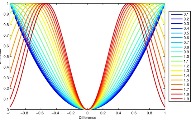
Fig. 1 The cosine dissimilarity

measure with changingα. (The distance is normalized for illustration purposes)

Ding et al.2006; Kwak2008; Ke and Kanade2003,2005; de la Torre and Black2003; Chin et al.2006) Euler-PCA allows for an efficient incremental implementation – contrary to KPCA approaches with standard kernels such

as GRBF we show that there exists an efficient way for pre-image computation without solving optimization problems.

In the experiments we show that the proposed Euler-PCA not only possesses these favorable properties but also out-performs the state-of-the-art.

Finally we note that compared to Tzimiropoulos (2012), our proposed method neither relies on the statistics of the gradient orientation differences nor restricts itself to the do-main of gradient orientations in general. Our work is a learn-ing method directly derived from the correlation method of Fitch et al. (2005), while Tzimiropoulos (2012) can be seen as the learning method derived from the analysis of the orientation correlation function presented in Tzimiropoulos (2010).

The rest of the paper is organized as follows. In Sect.2we introduce the cosine-based dissimilarity measure that forms the basis of the proposed Euler-PCA. In Sect.3we formulate the proposed Euler-PCA and discuss some of its properties. Experimental results are presented in Sect.4. Finally, con-clusions are drawn in Sect.5. Video sequences of our results are provided in the supplementary material.

2 Cosine-Based Dissimilarity

Let xj be thep-dimensional vector obtained by writing im-age Ij in lexicographic ordering. Motivated by the recent work in Fitch et al. (2005) on robust correlation-based

trans-lation estimation, we replace the2-norm with the following dissimilarity measure

d(xj,xq)= p

c=1

1−cosαπxj(c)−xq(c)

, (6)

where the pixel values of the corresponding imagesIj,Iq are represented in the range [0,1] and α∈R+. Figure1 visualizes the dissimilarity function with changing values for α. A small value forα results in a function which re-sembles the2-norm. With increasingα, the effect of large distances possibly caused by outliers is reduced. In general, αrepresents the frequency of the cosine and is optimized to suppress the values caused by outliers.

As noted in Fitch et al. (2005), for pixel intensities in the range[0,1], (6) is equivalent to Andrews’ M-Estimate. In particular, the influence function of the kernel, i.e. the derivative of the kernel, is equivalent to Andrews’ influence function, which is given by

ψ (r)=

sin(π r) if −1≤r≤1

0 otherwise. (7)

The Fast Robust Correlation (FRC) scheme in Fitch et al. (2005) utilizes (6) and, unlike2-based correlation, is able to estimate large translational displacements in real images while achieving the same computational complexity.

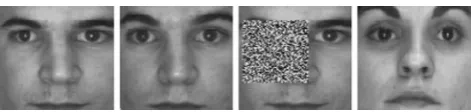
Prior to formulating the proposed PCA, let us consider a motivating example in which different dissimilarity mea-sures are applied to the images shown in Fig.2. As can be seen in Table 1, the 2-norm associates a smaller distance between the original image and an image from a different subject. The distance between the original and the same image with occlusion is larger. In contrast, the use of the cosine-based measure2 results in a large distance between the original image and the image of a different person.

Fig. 2 Example motivating the use of the cosine-based dissimilarity

measure. Shown from left to right are the original image, a second image of the same subject, an occluded version of the original image and an image of another subject

Table 1 Comparison of normalized dissimilarity measures

2-Norm Cosine measure Same subject 0.979×10−3 13.404×10−3 Occluded 1.96×10−3 _33.576×10−3 Different subject 1.63×10−3 34.599×10−3

3 Euler-PCA (e-PCA)

3.1 Batch Version

In this section we first present Euler-PCA and introduce its representation as both KPCA and linear PCA with special features.

Euler-PCA is a KPCA which utilizes the robust dissim-ilarity in (6). It is also based on the Euler representation of complex numbers. More specifically, we map the intensity values xjnormalized in[0,1]onto the complex representa-tion zj∈Cp, where

zj= 1 √ 2 ⎡ ⎢ ⎣

eiαπxj(1) .. . eiαπxj(p)

⎤ ⎥

⎦=√1

2e

iαπxj_{. (8)}

The values zj can be thought of as the special features in our version of PCA. To show the relationship between (8) and (6), let us defineθjαπxjand then apply the2-norm

zj−zq2F = 1

2cos(απxj)+isin(απxj)

−cos(απxq)+isin(απxq) 2 F

=

p

c=1

1−cosθj(c)−θq(c)

=d(xj,xq). (9)

This suggests that our KPCA can be defined by first ap-plying the explicit mapping of (8) and then using standard linear complex PCA. Because of (8), we coin this approach as Euler-PCA. Notice that forα <2, this mapping is one-to-one. In this case, this gives rise to fast pre-image com-putations via the ∠-operator, which returns the angle of a complex number. More specifically, after reconstruction (or de-noising) in the feature space has been performed, we can

Algorithm 1 ESTIMATING THE PRINCIPAL SUBSPACE Input: A set ofnimagesIj,j =1, . . . , n, ofppixels, the

numbermof principal components and parameterα. Output: The principal subspace B and eigenvaluesΣ.

1: RepresentIj in the range[0,1]and obtain xj by writing Ij in lexicographic ordering.

2: Compute zj using (8) and form the matrix of the trans-formed data Z= [z1· · ·zn] ∈Cp×n.

3: Compute the kernel matrix K=ZH_Z∈Cn×n _{and find} the eigendecomposition of K=UΛUH.

4: Find them-reduced set, Um∈Cn×mandΛm∈Rm×m. 5: Compute B=ZUmΛ−

1 2

m ∈Cp×mandΣ=Λ 1 2 m. 6: Reconstruct usingZ˜ =BBH_Z.

7: Fast pre-image computation: go back to the pixel do-main usingX˜ =∠_απZ˜.

Algorithm 2 EMBEDDING OF NEW SAMPLES

Input: The principal subspace B andαof Algorithm1, as well as a new imageI ofppixels.

Output: The embedding in subspace and pixel domain,z˜ andx respectively.˜

1: RepresentI in the range[0,1]and obtain x by writing I in lexicographic ordering.

2: Find z using (8) and reconstruct asz˜=BBHz.

3: Fast pre-image computation: go back to the pixel do-main usingx˜=∠_απz˜.

go back to the pixel domain using the∠-operator. Finally, high-dimensional data can be readily handled by using The-orem1(a proof can be found in AppendixA).

Theorem 1 Define matrices A and B such that A=ΦΦH

and B=ΦHΦ, where.H computes the complex conjugate transposition of a matrix. Let UA and UB be the

eigen-vectors corresponding to the non-zero eigenvaluesΛA and ΛB of A and B, respectively. Then, ΛA=ΛB and UA=

ΦUBΛ− 1 2 A .

The complete Euler-PCA is given in Algorithm1and Al-gorithm2.

k(xj,xq)= 1 2

p

c=1

cosαπxj(c)−xq(c)

−i1 2

p

c=1

sinαπxj(c)−xq(c)

. (10)

With the KPCA interpretation of the proposed method the strategy for reconstruction in the input space becomes less apparent. In the following section, we present the recon-struction by means of pre-image computation (Kwok and Tsang2004; Mika et al.1999) (a recent survey on pre-image computation problems can be found in Honeine and Richard (2011)). Then, we put our suggested approximationx˜=∠_απz˜ of Algorithms1 and2 for going back to the pixel domain (input space) in the context of pre-image computation and we derive a closed form to the approximation error.

3.2 Pre-image Computation

The optimization problem (5) for the proposed kernel can be reformulated as

˜

x=arg min ˇ

x

φ (x)ˇ −BBHφ (x)2_F

=arg min ˇ

x

k(x,ˇ x)ˇ +φ (x)HBBHBBHφ (x)

−φ (x)ˇ HBBHφ (x)−φ (x)HBBHφ (x)ˇ =arg min

ˇ

x −φ (x)ˇ H

BBHφ (x)−φ (x)HBBHφ (x)ˇ

=arg max ˇ

x

Reφ (x)ˇ HBBHφ (x), (11)

where Re(.) extracts the real part of a complex number and Im(.) the corresponding imaginary. Note, in KPCA the projection matrix is represented as a linear combination B=XφB, where X˜ φ= [φ (x1)· · ·φ (xn)]. Then, by setting

t= ˜BB˜H

⎡ ⎢ ⎣

k(x1,x) .. . k(xN,x)

⎤ ⎥ ⎦

the optimization problem (11) can be reformulated as

˜

x=arg max ˇ

x

Rek(x,ˇ x1) . . . k(x,ˇ xn)

t

=arg max ˇ

x

Rek(x,ˇ x1) . . . k(x,ˇ xn)

Re(t)

−Imk(x,ˇ x1) . . . k(x,ˇ xn)

Im(t)

=arg max ˇ

x n

j=1 p

c=1

cosαπx(c)ˇ −xj(c)

Ret(j )

+sinαπx(c)ˇ −xj(c)

Imt(j ) =arg max

ˇ

x f (x).ˇ (12) The standard way to optimize (12) is by gradient ascent (i.e. an update of the formxˇt= ˇxt−1+∇f (xˇt−1)(Mika et al.

1999)). Hence, we need to compute the partial derivatives ∂f

∂x(c)ˇ for all pixels as

∂f

∂x(c)ˇ = −απ N

j=1

Ret(j )sinαπx(c)ˇ −xj(c)

+απ N

j=1

Imt(j )cosαπx(c)ˇ −xj(c)

. (13)

Using (13),∇f can be concisely written as

∇f (x)ˇ = −Im(zˇz1) . . .Im(ˇzzn)

⎡ ⎢ ⎣ Re(t(1)) .. . Re(t(n)) ⎤ ⎥ ⎦

+Re(zˇz1) . . .Re(zˇzn)

⎡ ⎢ ⎣ Im(t(1)) .. . Im(t(n)) ⎤ ⎥ ⎦,(14)

whereis the element-wise product between vectors,ˇz is the transformφ (x)ˇ in (8) and¯.computes the complex conju-gate of a vector x. Unfortunately, the above procedure can be quite computational expensive for large databases (the order for recoveringK pre-images isO(μpKn)whereμis the number of steps until convergence).

In contrast, Algorithm1and2we have proposed a very fast way for approximating pre-images by

˜ x= 1

π α∠BB H

z. (15)

In the context of pre-image computation the error of this approximation canx can be analytically computed by sub-˜ stituting (15) into (8) and the result into (5) (details can be found in Appendix B)

φ (x)ˇ −BBHφ (x)2_F =√1 2e

i∠BBH_z

−BBHz 2

F

=√1 21−R

BBHz 2

F

, (16)

whereR(b)= [Re(b(c))2_+Im(b(c))2_{] is a vector} con-taining the magnitude of the elements in b and 1 is a vec-tor of ones. Finally, due to the invertibility of the proposed mapping (8) for 0≤α <2, in the case of B containing all eigenvectors that correspond to non-zero eigenvalues, it can easily be shown that the pre-image approximation using (15) is optimal for the training set (i.e. (16) is equal to zero).

3.3 Incremental Learning

Algorithm 3 INCREMENTALSUBSPACEESTIMATION Input: The principal subspace Bt−1∈ Cp×m, the

corre-sponding eigenvaluesΣt−1∈Rm×m, a set of new im-ages{In+1, . . . , In+a}, the numbermof principal com-ponents and parameterα.

Output: The new subspace Bt and eigenvaluesΣt. 1: From set {In+1, . . . , In+a} compute the matrix of the

transformed data Zδ= [zn+1· · ·zn+a].

2: Compute B δ=orth(Zδ−Bt−1B_tH₋1Zδ)and form L= Σt−1Bt−1HZδ

0 BH_δ Zδ

.

3: Compute Lsvd= ˆBΣˆVˆH_{and obtain them-reduced setB}ˆ m andΣˆm.

4: Compute Bt= [Bt−1Bδ] ˆBmand setΣt= ˆΣm.

PCA in a non-linear subspace defined by an explicit map-ping. We assume that the subspace Bt−1 of step t −1 is given by the SVD of Zt−1

Zt−1≈Bt−1Σt−1VHt−1=Zt−1UmΛ− 1 2 m Λ

1 2

mUHm, (17)

where UmΛmUHm is them-reduced eigenvalue decomposi-tion of ZH_t−1Zt−1. For the update, we want to find the SVD of the concatenated sample matrix, build from Zt−1, and the new mapped samples Zδ,

Zt= [Zt Zδ] ≈

Bt−1Σt−1VH_t−1 Zδ

. (18)

We reformulate (18) as

Zt≈ [Bt−1 Bδ]

Σt−1 BH_t−1Zδ 0 BH_δ Z

VH_t−1 0

0 I

, (19)

where Bδ=orth(Zδ−BBHZδ)contains the new compo-nents, which are not included in the current subspace Bt−1. Finally, the SVD of

L=

Σt−1 BH_t−1Zδ 0 BH_δ Z

= ˆBΣˆVˆH (20)

is all that is required for the update. With the m-reduced eigenspaceBˆm andΣˆmof L, we find Bt= [Bt−1 Bδ] ˆBm andΣ= ˆΣm. Algorithm3summarizes the main steps.

Note that existing methods for incremental KPCA in which the mapping is in general unknown are computation-ally expensive and inexact. For example in Chin and Suter (2007), to ensure constant execution speed, a set of pre-images are found to approximate the data matrix by solv-ing an extra optimization problem similar to (5). The draw-backs of this are twofold: (i) the reduced set representation provides only an estimate to the exact solution and (ii) the proposed optimization problem for finding the reduced set inevitably increases the complexity of the algorithm. On the other hand, since in our case, the mapping is explicit and does not increase the dimensionality we can represent the data matrix directly in feature space. This eliminates the

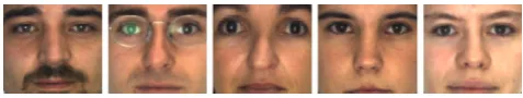
Fig. 3 Cropped example images from the AR Database (Martinez and

Benavente1998)

need to introduce an additional optimization problem, mak-ing the incremental version of Euler-PCA both fast and ex-act.

4 Experiments

4.1 Image Reconstruction Under Noise

In this section we evaluate the robustness of Euler-PCA (e-PCA) for the application on image de-noising based on subspace-based image reconstruction. For comparison, we select standard PCA, R1-PCA (Ding et al.2006), PCA-L1 (Kwak2008) and HQ-PCA (He et al.2011), which repre-sents the state-of-the-art, as well as, standard Kernel PCA de-noising with a GRBF KPCA (denoted by G-KPCA) and pre-image computation using (15) (denoted bye-PCA-GA). The parameters of R1-PCA, PCA-L1 and HQ-PCA follow (Ding et al.2006; Kwak2008; He et al.2011) respectively. We choose the convergence criterion for R1-PCA, PCA-L1 and HQ-PCA to be based on the norm difference between two successive subspace estimations. The maximum differ-ence is constrained not to exceed 10−8, unless a maximum of 50 iterations is reached. For the optimization of G-KPCA variance of the Gaussian kernel we tried two standard ap-proaches, but for compactness we always report the best results. In the first approach we set the variance equal to

1 n(n−1)

n

j,qxj−xq2where xj, xq are the training sam-ples (Kwok and Tsang2004). In the second method we ap-plied a cross-validation strategy in the training set for se-lecting the variance. For all methods that employ a gradi-ent descgradi-ent (or ascgradi-ent) for image computation the pre-images were initialized with all pixel intensities equal to 0.5. Finally, the methods were considered to have converged ifˇxt− ˇxt−1F ≤0.01 for two successive iterationst and t−1.

Our data set consists of a subset of the popular AR Database (Martinez and Benavente1998). In particular, we use a total of 100 images of size 101×91 of different sub-jects as shown in Fig.3.

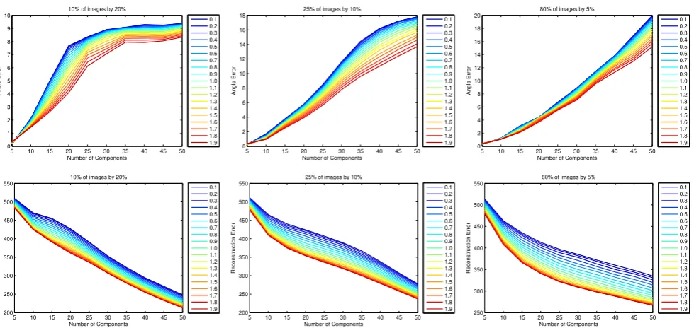
Fig. 4 Angular error (top) and reconstruction error (bottom) for different values forα

2011; Kwak2008). In particular, forntest samples, we com-pute

er(m)= 1 n

n

j=1

x

orig j −

m

l=1

bcor_l bcor_l Txcor_j

(21)

where xorig_j and xcor_j represent the original and the training image respectively, Bcor _{= [b}cur

1 · · ·bcurm ] ∈Rp×mis the es-timated subspace of the corrupted data and mdenotes the number of components used. For the methods that use pre-images for approximating the reconstruction error (21) is re-formulated as

er(m)= 1 n

n

j=1

_xorig j − ˜x

cor

j (m) (22)

wherex˜cor_j (m)is the pre-image associated with the recon-struction usingmcomponents in the feature space (i.e. solv-ing optimization problems (5) and (11) usingmcomponents for matrix B). Note, that for Euler-PCA de-noising is per-formed by calculating pre-images in two ways: by applying the∠-operator and by the gradient ascent optimization. We denote the latter method ase-PCA-GA. The calculation of pre-images for G-KPCA is also performed in a similar fash-ion.

Additionally we use the angular error between the cor-rupted subspace Bcor (learned from the corrupted training set) and the uncorrupted subspace Borig= [borig₁ · · ·borigm ] ∈ Rp×m _{(learned from the original images) as follows} (Gu-nawan et al.2005; Krzanowski1979)

ea(m)=m− m

l=1 m

s=1

cos2borig_l ,bcor_s . (23)

For the nonlinear methods Borig _{and B}cor _{are in the} fea-ture space but still cos(borig_l ,bcor_s )can be efficiently com-puted using the kernel. In contrast to the reconstruction error which introduces an inherent error due to the chosen number of components, the angle error shows the difference caused by the outliers directly.

4.1.1 Synthetic Corruptions

In this experiment, a percentage of training images is cor-rupted by randomly placed patches of random pixel noise as shown in Fig.9. We vary both the number of corrupted images and the size of the corrupted area. For convenience, we say “a % of images byb %” to denote thata% of the images in our training set was corrupted by randomly placed patches the size of which isb% of the total image size. After training we analyze the results based on the reconstruction and angle errors.

In our experiments, we tested the 5 different methods for 7 setups. These setups can be summarized into three types:

– Type (i): large occlusions on few images (e.g. 5 % of

im-ages by 30 % and 10 % of imim-ages by 30 %)

– Type (ii): medium sized occlusions on a few images (e.g. 10 % of images by 20 %, 15 % of images by 10 % and 25 % of images by 10 %)

– Type (iii): small occlusions on many images (e.g. 80 % of

images by 5 % and 85 % of images by 5 %)

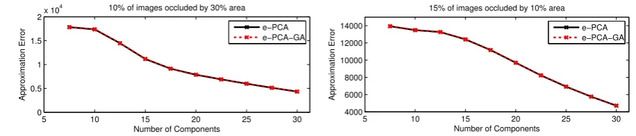
Fig. 5 Approximation error betweene-PCA ande-PCA-GA

for all the experiments in this paper. This is in contrast with GKPCA which includes an extra step for finding the opti-mum variance.

In order to test whether the pre-image approximation us-ing (15) is a valid choice we calculated the attained mini-mum of optimization problem (11), after performing the gra-dient ascent, and we compare it with the error given in (16). For all experiments the error of the fast pre-image approxi-mation resulted in similar or lower errors. A representative example can be found in Fig.5where the pre-image approx-imation error is plotted versus the number of components. It is evident that both the pre-image computation methods pro-duce similar errors (here we have to note that the pre-image approximation error is different than the reconstruction er-ror in (22) since the former is in the feature space while the latter is in the input space).

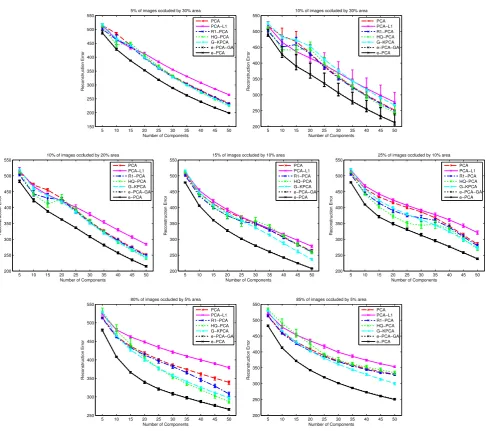
Figure 6 shows the reconstruction errors of all tested methods. In type (i) and (ii), HQ-PCA performs well for few components, while R1-PCA performs worse than HQ-PCA but better than standard PCA. As the number of components increases, PCA, R1-PCA and HQ-PCA perform the same. PCA-L1 performs well only for a small number of compo-nents. G-KPCA performs as good as HQ-PCA. In all exam-ples, both versions of the proposed Euler-PCA performs the best even for a large number of components.

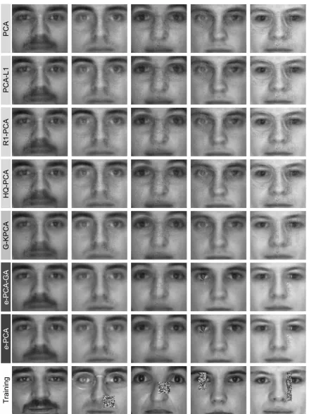
More distinctions between the tested methods are observ-able for type (iii). Here, PCA and R1-PCA have similar per-formance, up to 30 components, after which R1-PCA out-performs standard PCA. Similar conclusions can be drawn for HQ-PCA. Again, Euler-PCA outperforms all other meth-ods. Qualitative reconstruction results can be seen in Fig.9. As it can be seen, our method is able to largely suppress such outliers.

The angular error results reveal different performance as it can be seen in Fig.7. HQ-PCA outperforms PCA-L1 only for a large number of components. R1-PCA and standard PCA perform similarly. G-KPCA seems to perform the sec-ond best. This suggest that the performance improvement obtained for G-KPCA might be due to the fact that, for this experiment, the calculation of pre-images is not necessary. It seems that this calculation (as required by the reconstruction experiment) might be problematic. Once more, the proposed Euler-PCA performs best.

4.1.2 Hand Occlusions

In our second experiment we use skin-like occlusions to ver-ify the results of the previous section. In particular, we oc-clude a subset of the training data with hand signs of the American fingerspelling alphabet3(Fig.8). The chosen sign (letter), its orientation and its position are randomized, and the skin color is adjusted to fit the subject.

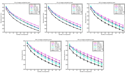
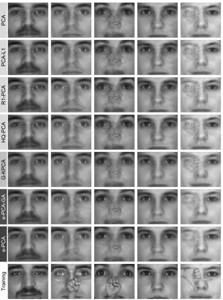
Figure10shows the reconstruction error and Fig.11the angular error. As before, HQ-PCA and G-KPCA outperform R1-PCA and standard PCA. Again, PCA-L1 performs the worst. Euler-PCA performs the best. Slightly different re-sults can be observed for the angular error. In contrast to our previous setup, here, R1-PCA, PCA and Euler-PCA per-form similarly well. Again, G-KPCA perper-forms very well for this experiment. However, HQ-PCA and PCA-L1 seem to perform worse. The corruption by hand occlusions is much more subtle than the one introduced by the random pixel patches. Therefore, PCA and R1-PCA achieve a similar per-formance to Euler-PCA in terms of angular error. Nonethe-less, the general trend follows our results of the previous section. Euler-PCA works well in terms of both reconstruc-tion and angular error. Figure12shows an example of the reconstruction quality.

4.2 Object Tracking

We evaluate the incremental version of Euler-PCA for the application of visual tracking. The aim of a visual track-ing system is to locate a predefined target object on every frame of a video sequence. Automatic systems span a wide range of applications, such as traffic monitoring (Kamijo et al.2000; Hsieh et al.2006), surveillance (Haritaoglu et al. 2000; Collins et al.2001), video retrieval and summarization (Luo et al.2003), vehicle navigation (Hashima et al.1997; Fraundorfer et al.2007), driver assistance (Handmann et al. 1998; Avidan 2004), human computer interaction (Wren et al.1997; Liwicki and Everingham2009) and face analy-sis (Gunes and Pantic2010; Cohn et al.1999). Many track-ing algorithms indicate that an adaptive approach based on

Fig. 6 Reconstruction error with different rates of occluded images. Here, the mean value over 10 executions with different random patches is

shown. Variance is indicated by error bars

online learning is advantageous to fixed appearance mod-els learned offline (Babenko et al.2011; Ross et al.2008; Mei and Ling2009). We evaluate the tracking performance of Euler-PCA based on precision and accuracy and then compare it to four other state-of-the-art holistic trackers.

4.2.1 Framework

We combine the appearance model learned by the incremen-tal version of Euler-PCA with a motion affine transforma-tion and a particle filter, in a similar fashion to Ross et al. (2008) and Chin and Suter (2007). In general, a particle fil-ter calculates the posfil-terior of a system’s states based on a transition model and an observation model. In our tracking framework, the transition model is described as a Gaussian

Mixture Model around an approximation of the state poste-rior distribution of the previous time step,

pAi_t|A1_t−:P₁= P

i=1

w_ti₋₁NAt;Ait−1,Ξ

(24)

Fig. 7 Angular error with different rates of occluded images. Here, the mean value over 10 executions with different random patches is shown.

Variance is indicated by error bars

probable sample is selected as the stateAbest_t at timet. Thus, the estimation of the posterior distribution is an incremental process and utilizes a hidden Markov model which only re-lies on the previous time step.

Our observation model computes the probability of a sample being generated by the learned eigenspace in the ap-pearance model. We assume that the probability of the ob-servation, given the tracking parameters att, is analogous to an exponential as

pφyi_t|Ai_t∝e−γφ (yit)−BBHφ (yit)2F

=e−γzit−BBHzit2F (25) where yi_tis the observation vector at timetof location Ai_t, zi_t is its mapping from (8) andγ is the parameter that controls

Fig. 8 Examples of the corruptions in the training data

the spread. Algorithm4describes the proposed visual track-ing framework, which we coin Euler Kernel Tracker (eT).

4.2.2 Results

Fig. 10 Reconstruction error with different rates of hand occluded images. Here, the mean value over 10 executions is shown. Variance is indicated

by error bars

Algorithm 4 EULERKERNELTRACKER ATTIMEt Input: The previous eigenspace Bt−1, Σt−1, locations

A_t1₋:P₁, weightsw1_t−:P₁, image frame It∈ [0,1]andα. 1: DrawP particles A1_t:P fromp(Ai_t|A1_t−:P₁)as in (24). 2: Take all image patches from It which correspond to

par-ticles A1:P

t and order their values lexicographically to form vectors y1_t:P.

3: Form the mapping z1t:P as in (8) and compute the prob-ability of each particlep(zi

t|Ait)as in (25) and extract the weightsw1_t:P.

4: Choose Abestt and zbestt as the affine transform and fea-tures of the particle with the largest weight.

5: Using zbest_t update the subspace by applying Algo-rithm3in a batch after a certain number of frames (5 in our implementation).

art tracking approaches: IVT4 (Ross et al.2008), IKPCA5 (Chin and Suter2007), the L1 tracker6_{(Mei and Ling2009)}

and MIL tracker7(Babenko et al.2011),

We evaluate the performance of all methods on 8 very popular video sequences (subsets of which are used in Babenko et al. (2009,2011), Ross et al. (2008), Mei and Ling (2009), Comaniciu et al. (2003)),Vi,i=1, . . . ,8, with drastic changes of the target’s appearance including pose variation, occlusions and non-uniform illumination.8 Quali-tative results are illustrated in Fig.13.

VideoV1is provided along with 7 annotated points which indicate the ground truth. We also annotate 3–7 fiducial points for the remaining sequences (Liwicki et al. 2012). Our quantitative performance evaluation is based on the root mean square (RMS) error between the true and the esti-mated locations of these points (Ross et al. 2008). Simi-larly to (Babenko et al.2011), we additionally present pre-cision plots which visualize the quality of the tracking. Such graphs show the percentage of frames in which the target was tracked with an RMS error less than a certain threshold. In our experiments, all trackers use an affine motion model with a fixed number of drawn particles (800 parti-cles). We attempt to optimize the performance of all

track-4_{The Matlab implementation is publicly available athttp://www.cs.} toronto.edu/~dross/ivt/.

5_{The Matlab implementation of the IKPCA was kindly provided by the} authors of the paper.

6_{The implementation is publicly available athttp://www.ist.temple.} edu/~hbling/code_data.htm.

7_{The implementation (only for translation motion model) is publicly} available at http://vision.ucsd.edu/~bbabenko/project_miltrack.shtml, we carefully modified it in order to support an affine motion model in a particle filter framework.

8_VideosV

4andV5are available athttp://vision.ucsd.edu/~bbabenko/ project_miltrack.shtml and the remaining videos are published at http://www.cs.toronto.edu/~dross/ivt/.

ers using video-specific parameters. That is, for each tracker and video, we found the parameters which gave the best per-formance in terms of robustness (i.e. how many times the tracker went completely off) and accuracy (measured by the RMS error).

Apart from the L1 tracker (for which the resolution of the template increases geometrically the complexity) the track-ing template was chosen to be of resolution of 32×32. All trackers were optimized with respect to (wrt) the variance of the Gaussian from which we sample the particles. Addition-ally to the variance of the Gaussian, which is common for all the systems, we optimizeeT, IVT and IKPCA wrt the num-ber of components and the spreadγ. ForeT the value forα

is fixed to 1.9. IKPCA was also optimized wrt the variance of the Gaussian RBF function. Furthermore, we optimized L1 wrt the resolution of the templates (the tracking becomes impractical for particles larger than 20×20). For MIL we optimized wrt the parameters mentioned in Babenko et al. (2011) (e.g. the number of positives in each frame, the num-ber that controls the sampling of negative examples, the learning rate for the weak classifiers).

For these versions of the trackers, Table2lists the mean RMS error for all sequences and the average frame rate of each tracker,9while Fig.14plots the RMS error as a func-tion of the frame number. Figure15shows the accuracy in terms of precision plots. Qualitative tracking results for all methods are shown in Fig.13. The videos are provided as part of the supplementary material.

In general, the robustness of eT is similar to IVT, al-though,eT performs the best in terms of precision for most videos. MIL and L1 are more robust and track the target inV5 successfully. However, particularly visible in the re-sults forV8, L1 is not precise for outliers caused by mo-tion blur. MIL is based on a bag of features approach, and consequently is inherently unprecise. IKPCA fails for all se-quences. Our tracker performs very well particularly forV4 in which the target undergoes many prolonged partial occlu-sions. Thee-PCA’s robustness successfully suppresses these outliers for this video sequence. In terms of efficiency, IVT ande-PCA operate in the highest frame rate, while all other methods operate in less than one frame per second.

4.3 Background Modeling

Background modeling algorithms aim to estimate the back-ground of a scene from a video sequence usually captured with a static camera. This problem can be naturally tack-led using PCA (Oliver et al.2000): the frames of the video are used to estimate a low dimensional subspace. Then the

Fig. 15 Tracking precision for each video sequence

Table 2 Mean RMS error for

general tracking, and tracking rate. “(lost)” indicates sequences in which the tracker clearly does not follow the target throughout

V1 V2 V3 V4 V5 V6 V7 V8 Fames/second

IVT 6.82 (lost) 4.07 10.79 (lost) 3.31 1.78 2.62 3.157

IKPCA (lost) (lost) (lost) (lost) (lost) (lost) (lost) (lost) 0.832 L1 6.17 (lost) 2.87 11.10 12.68 9.53 1.62 13.58 0.076 MIL 16.95 (lost) 13.61 14.62 37.56 12.73 4.14 23.87 0.129 eT 5.14 (lost) 3.68 4.68 (lost) 3.04 1.73 2.44 2.935

Table 3 Maximum similarity

of Fig.16 Airport Bar Lobby Curtain Escalator Fountain Mall Campus Water

PCA 0.540 0.503 0.600 0.686 0.442 0.508 0.545 0.286 0.767

PCA-L1 0.540 0.504 0.604 0.671 0.442 0.548 0.540 0.286 0.767 R1-PCA 0.474 0.499 0.607 0.727 0.428 0.563 0.551 0.294 0.503 HQ-PCA 0.486 0.498 0.615 0.755 0.422 0.558 0.544 0.292 0.776

e-PCA 0.584 0.533 0.609 0.747 0.479 0.534 0.563 0.304 0.774

Table 4 Execution time

required to compute the appearance model for the last frame of each video sequence (5 components)

Airport Bar Lobby Curtain Escalator Fountain Mall Campus Water PCA 0.003 s 0.002 s 0.003 s 0.002 s 0.002 s 0.002 s 0.002 s 0.010 s 0.003 s PCA-L1 12.4 s 9.5 s 5.1 s 6.3 s 21.7 s 1.2 s 3.3 s 9.7 s 1.4 s R1-PCA 123.0 s 120.0 s 44.7 s 124.9 s 233.0 s 12.4 s 35.9 s 182.8 s 8.1 s HQ-PCA 2663.4 s 930.8 s 365.8 s 3106.8 s 2536.7 s 36.7 s 91.0 s 282.3 s 71.8 s e-PCA 0.007 s 0.006 s 0.006 s 0.006 s 0.006 s 0.006 s 0.006 s 0.026 s 0.006 s

background corresponding to each of the video frames is ob-tained by reconstructing the frame from this subspace. Once

Fig. 16 Similarity with changing number of components

For our evaluation, we used the popular data set from Li et al. (2004). The set consists of 9 videos including illu-mination changes, indoor/outdoor environments as well as dynamic background changes. The ground truth for fore-ground/background pixels of 20 randomly selected frames for each video is also provided Li et al. (2004). Standard PCA, PCA-L1, R1-PCA and HQ-PCA are used for compar-ison. We present quantitatively and qualitatively results. For the former case, we use the similarity measure (Maddalena and Petrosino2008)

Similarity= tp

tp+fp+fn (26)

where tp, fp and fn are the numbers of correctly labeled foreground, falsely labeled background and falsely labeled foreground pixels respectively. The setup for PCA, PCA-L1, R1-PCA, HQ-PCA ande-PCA is similar to Sect.4.1.

Fur-thermore, PCA and Euler-PCA is updated incrementally for each frame during learning.

We used the complete set of preceding frames to train the models (e.g. for frame 100, the preceding 99 frames are used for the appearance model), and for each video, we eval-uate the similarity for the frames in which the ground truth is provided. The mean similarity, as a function of the num-ber of components, is plotted in Fig.16. The best similarity value for each method and video is summarized in Table3, while Fig.17shows the performance qualitatively. In gen-eral,e-PCA performs the best in 5 out of 9 sequences, and the second best for 3. The results of the other methods vary for each sequence. The videos are provided in the supple-mentary material.

Fig. 17 Examples of background modeling for each video and each method. In the results, black indicates correctly predicted background, blue

computer with an Intel core i7 870 processor at 2.93 GHz and 8 GB RAM. PCA and Euler-PCA can be updated incre-mentally, making their running time less than a second for all sequences. In contrast, the other methods require a recal-culation of the complete appearance model for each frame. Consequently, these methods are much slower.

5 Conclusion

We introduce a fast, direct and robust approach to PCA. The proposed Euler-PCA allows for fast incremental computa-tion and retains the favorable properties of standard2-norm PCA, while suppressing outliers. Our experiments show that Euler-PCA achieves promising results for the applications of face reconstruction, object tracking and background model-ing. In future work we intend to introducee-PCA to a range of further applications in human computer interaction, com-puter vision and pattern recognition.

Acknowledgements The research presented in this paper is sup-ported in part by the European Research Council (ERC) under the ERC Starting Grant Agreement ERC-2007- StG-203143 (MAH-NOB). The work of S. Liwicki is supported by the Engineering and Physical Science Research Council DTA Studentship. The work of G. Tzimiropoulos is currently supported in part by the European Community’s 7th Framework Programme FP7/2007-2013 under Grant Agreement 288235 (FROG).

Appendix A: Proof of Theorem1

Proof Given A=ΦΦH and B=ΦHΦ their eigenspaces is provided by A=UAΛAUHA and B=UBΛBUHB. Fur-thermore, UH

AUA=UHBUB=I. Let us define matrix M=

ΦUBΛ− 1 2

B . We get

MHAM=Λ− 1 2 B U

H

BΦHΦΦHΦUBΛ− 1 2 B

=Λ− 1 2 B U

H

BBBUBΛ− 1 2 B

=Λ− 1 2 B U

H

BUBΛBUHBUBΛBUHBUBΛ− 1 2 B

=Λ− 1 2

B ΛBΛBΛ

−1 2 B

=ΛB. (27)

Therefore,ΛA=ΛB and UA=M for non-zero

eigenval-ues.

Appendix B: Proof that _√1

2e

i_∠b_−b2 F=

1

√

2−R(b) 2 F

√1

2e

i∠b_−b 2

F

=

p

c=1

1 √

2e

i∠b(c)_−b(c)

2

=

p

c=1

1 √

2e i∠b(c)₋

Rb(c)ei∠b(c)

2

=

p

c=1

1 √

2−R

b(c) 2

=√1

21−R(b)

2

F

, (28)

whereR(b)= [Re(b(c))2_+Im(b(c))2_{] is a vector with} the magnitude of the elements of b and 1 is a vector of

ones.

References

Avidan, S. (2004). Support vector tracking. IEEE Transactions on

Pat-tern Analysis and Machine Intelligence, 1064–1072. doi:10.1109/ TPAMI.2004.53.

Babenko, B., Yang, M., & Belongie, S. (2009). Visual tracking with online multiple instance learning. In CVPR’09 (pp. 983–990). Babenko, B., Yang, M., & Belongie, S. (2011). Robust object

track-ing with online multiple instance learntrack-ing. IEEE Transactions

on Pattern Analysis and Machine Intelligence. doi:10.1109/ TPAMI.2010.226.

Candés, E., Li, X., Ma, Y., & Wright, J. (2009). Robust principal com-ponent analysis? Available at:http://arxiv.org/abs/0912.3599v1. Chin, T. J., & Suter, D. (2007). Incremental kernel principal component

analysis. IEEE Transactions on Image Processing, 1662–1674. doi:10.1109/TIP.2007.896668.

Chin, T., Schindler, K., & Suter, D. (2006). Incremental kernel SVD for face recognition with image sets. In FG’06 (pp. 461–466). Cohn, J., Zlochower, A., Lien, J., & Kanade, T. (1999). Automated

face analysis by feature point tracking has high concurrent validity with manual FACS coding. Psychophysiology, 35–43. doi:10.1017/S0048577299971184.

Collins, R., Lipton, J., Fujiyoshi, H., & Kanade, T. (2001). Algorithms for cooperative multisensor surveillance. In The IEEE (p. 89). doi:10.1109/5.959341.

Comaniciu, D., Ramesh, V., & Meer, P. (2003). Kernel-based object tracking. IEEE Transactions on Pattern Analysis and Machine

In-telligence, 564–577. doi:10.1109/TPAMI.2003.1195991. de la Torre, F., & Black, M. (2003). A framework for robust

sub-space learning. International Journal of Computer Vision, 117– 142. doi:10.1023/A:1023709501986.

Ding, D., Zhou, D., He, X., & Zha, H. (2006). R1-PCA: rotational invariant L1-norm principal component analysis for robust sub-space factorization. In ACM (pp. 281–288). doi:10.1145/1143844. 1143880.

Fitch, A., Kadyrov, A., Christmas, W., & Kittler, J. (2005). Fast robust correlation. IEEE Transactions on Image Processing, 1063–1073. doi:10.1109/TIP.2005.849767.

Fraundorfer, F., Engels, C., & Nistér, D. (2007). Topological map-ping, localization and navigation using image collections. In

In-tell. robots and systems (pp. 3872–3877).

Gunawan, H., Neswan, O., & Budhi, W. (2005). A formula for angles between subspaces of inner product spaces. Contributions to

Al-gebra and Geometry, 46(2), 311–320.

Gunes, H., & Pantic, M. (2010). Automatic, dimensional and continu-ous emotion recognition. International Journal of Synthetic

Emo-tion, 68–99. doi:10.4018/jse.2010101605.

Haritaoglu, I., Harwood, D., & Davis, L. (2000). W4: real-time surveillance of people and their activities. IEEE

Transac-tions on Pattern Analysis and Machine Intelligence, 809–830.

doi:10.1109/34.868683.

Hashima, M., Hasegawa, F., Kanda, S., Maruyama, T., & Uchiyama, T. (1997). Localization and obstacle detection for a robot for car-rying food trays. In Intell. robots and systems (pp. 345–351). He, R., Hu, B., Zheng, W., & Kong, X. (2011). Robust

princi-pal component analysis based on maximum correntropy cri-terion. IEEE Transactions on Image Processing, 1485–1494. doi:10.1109/TIP.2010.2103949.

Honeine, P., & Richard, C. (2011). Preimage problem in kernel-based machine learning. IEEE Signal Processing Magazine, 28(2), 77– 88.

Hsieh, J., Yu, S., Chen, Y., & Hu, W. (2006). Automatic traffic surveillance system for vehicle tracking and classification. IEEE

Transactions on Intelligent Transportation Systems, 175–187.

doi:10.1109/TITS.2006.874722.

Jolliffe, T. (2002). Principal component analysis (2nd edn.). Berlin: Springer.

Kamijo, S., Matsushita, Y., Ikeuchi, K., & Sakauchi, M. (2000). Traffic monitoring and accident detection at intersections. IEEE

Transactions on Intelligent Transportation Systems, 108–118.

doi:10.1109/6979.880968.

Ke, Q., & Kanade, T. (2003). Robust subspace computation using L1

norm (Tech. Rep. CMU-CS-03-172). Computer Science

Depart-ment, Carnegie Mellon University.

Ke, Q., & Kanade, T. (2005). Robust L1 norm factorization in the pres-ence of outliers and missing data by alternative convex program-ming. In CVPR’05 (pp. 739–746).

Krzanowski, W. (1979). Between-groups comparison of principal com-ponents. Journal of the American Statistical Association, 703– 707. doi:10.1080/01621459.1979.10481674.

Kwak, N. (2008). Principal component analysis based on L1-norm maximization. IEEE Transactions on Pattern Analysis and

Ma-chine Intelligence, 1672–1680. doi:10.1109/TPAMI.2008.114. Kwok, J., & Tsang, I. (2004). The pre-image problem in kernel

meth-ods. IEEE Transactions on Neural Networks, 15(6), 1517–1525. Levy, A., & Lindenbaum, M. (2000). Sequential Karhunen-Loeve basis

extraction and its application to images. IEEE Transactions on

Image Processing, 1371–1374. doi:10.1109/83.855432. Li, Y. (2004). On incremental and robust subspace learning. Pattern

Recognition, 1509–1518. doi:10.1016/j.patcog.2003.11.010. Li, L., Huang, W., Gu, I., & Tian, Q. (2004). Statistical modeling

of complex backgrounds for foreground object detection. IEEE

Transactions on Image Processing, 13(11), 1459–1472.

Liu, W., Pokharel, P., & Principe, J. (2007). Correntropy: proper-ties and applications in non-Gaussian signal processing. IEEE

Transactions on Signal Processing, 5286–5298. doi:10.1109/TSP. 2007.896065.

Liwicki, S., & Everingham, M. (2009). Automatic recognition of fin-gerspelled words in British sign language. In CVPR4HB’09, in

conj. with CVPR’09 (pp. 50–57).

Liwicki, S., et al. (2012). doi:10.1109/TNNLS.2012.2208654. Luo, Y., Wu, T., & Hwang, J. (2003). Object-based analysis and

inter-pretation of human motion in sports video sequences by dynamic Bayesian networks. Computer Vision and Image Understanding, 196–216. doi:10.1016/j.cviu.2003.08.001.

Maddalena, L., & Petrosino, A. (2008). A self-organizing approach to background subtraction for visual surveillance applications. IEEE

Transactions on Image Processing, 1168–1177. doi:10.1109/TIP. 2008.924285.

Martinez, A., & Benavente, R. (1998). The AR face database (Tech. Rep. #24). The Ohio State University.

Mei, X., & Ling, H. (2009). Robust visual tracking using L1 minimiza-tion. In ICCV’09.

Mika, S., Schölkopf, B., Smola, A., Müller, K., Scholz, M., & Rätsch, G. (1999). Kernel pca and de-noising in feature spaces. Advances

in Neural Information Processing Systems, 11(1), 536–542.

Nguyen, M., & de la Torre, F. (2009). Robust kernel principal compo-nent analysis. In Advances in NIPS (pp. 1185–1192).

Oliver, N., Rosario, B., & Pentland, A. (2000). A Bayesian computer vision system for modeling human interactions. IEEE

Transac-tions on Pattern Analysis and Machine Intelligence, 831–843.

doi:10.1109/34.868684.

Paulsen, V. (2009). An introduction to the theory of reproduc-ing kernel Hilbert spaces. Available at: http://www.math.uh. edu/~vern/rkhs.pdf.

Ross, D., Lim, J., Lin, R., & Yang, M. (2008). Incremental learning for robust visual tracking. International Journal of Computer Vision, 125–141. doi:10.1007/s11263-007-0075-7.

Tzimiropoulos, G. (2010). IEEE Transactions on Pattern Analysis and

Machine Intelligence. doi:10.1109/TPAMI.2010.107.

Tzimiropoulos, G. (2012). IEEE Transactions on Pattern Analysis and

Machine Intelligence. doi:10.1109/TPAMI.2012.40.

Turk, M., & Pentland, A. (1991). Eigenfaces for recognition. Journal

of Cognitive Neuroscience, 71–86. doi:10.1162/jocn.1991.3.1.71. Wren, C., Azarbayejani, A., Darrel, T., & Pentland, A. (1997).

Pfinder: real-time tracking of the human body. IEEE

Transac-tions on Pattern Analysis and Machine Intelligence, 780–785.