Benchmark results for testing adaptive finite element eigenvalue procedures

(1)

BENCHMARK RESULTS FOR TESTING ADAPTIVE FINITE ELEMENT EIGENVALUE PROCEDURES

STEFANO GIANI, LUKA GRUBIˇSI ´C, AND JEFFREY S. OVALL

Abstract. A discontinuous Galerkin method, with hp-adaptivity based on the approx-imate solution of appropriate dual problems, is employed for highly-accurate eigenvalue computations on a collection of benchmark examples. After demonstrating the effectivity of our computed error estimates on a few well-studied examples, we present results for sev-eral examples in which the coefficients of the partial-differential operators are discontinuous. The problems considered here are put forward as benchmarks upon which other adaptive methods for computing eigenvalues may be tested, with results compared to our own.

1. Introduction

In 2005 Betcke and Treffethen wrote an influential paper [9] on the accurate computation of eigenvalues and eigenvectors of the Laplacian in planar regions, which gave insight into several interesting phenomena of the spectral theory of the Laplace operator on such domains. The computational approach used in [9] was a new implementation of the classical method of particular solutions. The structure of this method is such that it does not permit a similar analysis for other divergence-type elliptic operators whose coefficients are not C∞ smooth. This class of problems includes many interesting multiphase examples such as photonic crystals and related problems, see [3, 26, 27] and in particular [18, Chapter 4]. A particular subclass of such problems are the so-called “jumping coefficient” problems for which the coefficients of the differential operators are piecewise smooth on some partition of the domain, but have jump discontinuities.

In the present work, we investigate a class of “jumping coefficient” problems using ex-ponentially-convergent hp-adaptive discontinuous Galerkin (hp-DG) methods, with error estimates based on the Dual Weighted Residual (DWR) approach which has been already used successfully [15, 14] to study the stability of fluid dynamics problems. We argue that hp-adaptive methods are highly-efficient for computing eigenvalues of “jumping coefficient” problems — in terms of computational cost per accurate digit — and give indication of why we claim high accuracy of our computations. In many cases we discuss the significance (in terms of applications) of the models which our problems represent. We suggest that the eigenvalue approximations, convergence rates, effectivities of the computed error estimates, and computational cost information which we report here provide ideal benchmarks for study other adaptive finite element procedures designed to address such eigenvalue problems.

The model eigenvalue problem considered in this paper is: (1.1) Au:=−∇ ·(A∇u) +V u = λu ,

2000Mathematics Subject Classification. Primary: 65N30, Secondary: 65N25, 65N15.

Key words and phrases. eigenvalue problem, finite element method, a posteriori error estimates .

(2)

on a bounded domain Ω⊂R2 _{and subject to a homogeneous Dirichlet boundary condition,}

i.e. u= 0 on∂Ω. Here,Adenotes the self-adjoint operator which is defined by this differential expression and we assume that the matrix-valued functionAis real symmetric and uniformly positive definite, i.e.

(1.2) 0< a ≤ ξTA(x)ξ ≤ a for all ξ∈R2 _with _|_ξ_|_{= 1 and all} _x_∈_Ω _.

The scalar potential V is real and bounded above and below by constants for allx∈Ω, i.e. (1.3) 0 < V ≤ V(x) ≤ V for all x∈Ω.

The family of problems (1.1) is representative for a much larger class of singular stiff problems, see [23, 38], which can be written in the following abstract formulation, for κ >1,

Aκu=λu,

(1.4)

hκ(u, v) =hb(u, v) +κhe(u, v), u, v ∈Dom(hb)⊂Dom(he).

(1.5)

Here we assume that the self-adjoint operator Aκ is defined by positive definite quadratic

forms hκ, he and hb in the sense of Kato [31], e.g. (A1/2κ u,A1/2κ v)L2 = h_κ(u, v), u, v ∈

Dom(hκ) = Dom(A1/2κ ). In this setting we assume that he has a large null space in order for

the problem to belong to the class of singular stiff problems. Problems with the structure (1.4)–(1.5) have applications in quantum mechanics, nano-optics, theory of vibrations of com-posite and porous materials and similar classes of singularly perturbed models. Furthermore, the differential expression (1.1) allows for a consideration of multi-scale eigenvalue problems for composite materials such as those from [12, 13]. More specifically, if A(x) = A(x+k) and V(x) =V(x+k) for all k∈Z2 _and _x_∈R2_{, one might condsider the family of problems}

(1.6) Aεu:=−∇ ·(A(·/ε)∇u) +V(·/ε)u = λu ,

for 0< ε≪1.

Both classes of problems (1.4) and (1.6) converge to well-defined limit problems asκ→ ∞

or ε → 0. Furthermore, the limit problems are frequently analytically soluble and posed only in a portion of the domain Ω. The computational challenge is to capture the transient behavior as the limiting procedure converges. In typical applications ε is small but nonzero and one is interested in capturing the oscillation and concentration properties of eigenvectors; whereas for large but finite κ one is often concerned with the tunneling properties, e.g. exhibiting exponential decay away from the domain where the limit problem is posed. One further difference between these problems is in the nature of the convergence. In the first case, we have that A−κ1 converges monotonically, which often leads to convergence of the resolvent

in norm. In the second case we do not have monotonicity properties of the sequence A−1 ε as

ε→0, so at best we can conclude that the resolvents converge strongly. In its most general case strong resolvent convergence does not guarantee the conservation of multiplicities of eigenvalues in the passage to the limit (see [31]). Problems involving the operator Aε will

not further be considered in this work; but we plan to return to this problem later, since the current state-of-the-art is to use numerical solutions on a very fine grid to test the convergence of a multi-scale numerical approximation method (cf. [12, Section 6] and [13]), and we believe that the approach put forth here has greater potential for efficiency.

The rest of the paper is structured as follows: In Section 2 we provide a detailed description of the hp-DG weak formulation of our model eigenvalue problem. Section 3 provides the background and basic results for the DWR error estimates which we employ. We describe,

(3)

in detail, two variants of the adaptive procedures used for our numerical experiments in Section 4. The bulk of the paper, Section 5, is devoted to presenting and discussing our benchmark results.

2. Formulation of the discontinuous Galerkin method

In recent years the discontinuous Galerkin (DG) methods for elliptic problems [4] have become increasingly popular. Some of the main reasons for this increase of interest in DG methods is that allowing for discontinuities across elements gives extraordinary flexibility in terms of mesh design and choice of shape functions. Additionally, hp-DG, which are based on locally refined meshes and variable approximation orders, have been shown to achieve tremendous gains in computational efficiency for challenging problems [24, 25, 29, 28].

Since we are going to construct sequences of adaptively refined shape-regular meshes, we denote the meshes by Tn, where n is the index of the mesh. The meshes Tn are partitions

of Ω ⊂ R2 _{into open triangles or quadrilaterals} _{_K_}_K_∈T_n_{. We also assume that, in the}

interior of each element K ∈ Tn, the positive definite matrix A and the potential V are

smooth. In presence of jumping coefficients, the jumps are aligned with the meshes used in this work. The diameter of an element K ∈ Tn is denoted by hK. Due to our assumptions

on the meshes, these diameters are of bounded variation, that is, there is a constant b1 ≥1

such that

(2.1) b−₁1 ≤hK/hK′ ≤b₁,

wheneverKandK′

share a common edge. We store the elemental diameters in the mesh size vector h={hK : K ∈ Tn}. Similarly, we associate with each element K ∈ Tn a polynomial

degree pK ≥ 1 and define the degree vector p = {pK : K ∈ Tn}. We assume that p is of

bounded variation as well, that is, there is a constant b2 ≥1 such that

(2.2) b−21 ≤pK/pK′ ≤b₂,

whenever K and K′

share a common edge.

For a partition Tn of Ω and a degree vector p, we define the hp-version discontinuous

Galerkin finite element spaceSn of real valued functions by

(2.3) Sn ={v ∈L2(Ω) : v|K ∈ PpK(K), K ∈ Tn},

where, if K is a triangle, PpK(K) is the space of polynomials on K of total degree less or

equal pK, otherwise if K is a quadrilateral, PpK(K) is the space of polynomials on K of

degree less or equal pK in each dimension.

Next, we define some trace operators that are required for the DG methods. To this end, we denote by EI(Tn) the set of all interior edges of the partition Tn of Ω, and by EΓ(Tn)

the set of all boundary edges of Tn. Furthermore, we define E(Tn) = EI(Tn)∪ EΓ(Tn). The

boundary∂K of an elementK and the sets∂K\Γ and∂K∩Γ will be identified in a natural way with the corresponding subsets ofE(Tn).

Let K+ _and _K−

be two adjacent elements of Tn, and κ ∈ EI(T_n) given by κ = ∂K+ ∩ ∂K−

. Furthermore, let v be a complex scalar-valued function, that is smooth inside each element K±

. By v±

, we denote the traces of v on κ taken from within the interior of K±

, respectively. Then, since we are dealing with jumping coefficients we need to use the

(4)

definition of the weighted average of the diffusive fluxA∇nv along κ∈ EI(T_n) introduced in [20]

{{A∇nv}}=ω

−

(A∇nv)

−

+ω+(A∇nv)+ ,

where

ω−

= n

t

K+A+n_K+

nt_K−A

−

nK−+nt

K+A+n_K+

, ω+= n

t K−A

− nK−

nt_K−A

−

nK−+nt

K+A+n_K+

,

where we denote by n_K± the unit outward normal vector of ∂K±, respectively. Similarly,

for a scalar function we have the following weighted average

{{v}}=ω−v++ω+v− . Then, the jump ofv across κ∈ EI(T_n) is given by

[[v]] =v+_n

K+ +v−n_K−,

[[A∇nv]] =AK+∇_nv+·n_K++A_K−∇_nv−·n_K−.

On a boundary edgeκ∈ EΓ(Tn), we set{{A∇nv}}=A∇nv and [[v]] = vn, withndenoting

the unit outward normal vector on the boundary Γ.

For a mesh Tn on Ω and a polynomial degree vector p, let Sn be the hp-version finite

element space defined in (2.3). We consider the (symmetric) weighted interior penalty dis-cretization [20] of (1.1): find (λn, un)∈R×Sn such that

(2.4) An(un, v) = λn(un, v) , for all v ∈Sn ,

with (un, un) = 1 and where

An(u, v) :=

X

K∈Tn Z

K

AK∇nu· ∇nv+V uv dr

− X

κ∈E₍Tn) Z

κ

{{A∇nv}} ·[[u]] +{{A∇nu}} ·[[v]]ds+

X

κ∈E₍Tn) Z

κ

c[[u]]·[[v]]ds,

(u, v) :=

Z

Ω

uv dr ,

here, ∇n denotes the element wise gradient operator andAK denotes the restriction of AK

ontoK. Furthermore, the function c∈L∞

(E(Tn)) is the discontinuity stabilisation function

that is chosen as follows: we define the functions h∈L∞

(E(Tn)) and p∈L∞(E(Tn)) by

h(r) :=

(

min(hK+, h_K−), r ∈κ ∈ E_I(T_n), κ=∂K+∩∂K−,

hK, r ∈κ ∈ EΓ(Tn), κ∈∂K ∩Γ,

p(r) :=

(

max(pK+, p_K−), r∈κ∈ EI(T_n), κ=∂K+∩∂K−,

pK, r∈κ∈ EΓ(Tn), κ∈∂K ∩Γ,

and set the penalty parameter to be

(2.5) c=γω+nt_K+A+n_K+

p2 h,

with a parameterγ >0 that is independent ofh,p,AK+ andA_K−. The parametercdefined

here is an hp-version of the weighted penalty parameter [20].

(5)

3. Goal-oriented a posteriori error estimation

In this section we introduce the a posteriori analysis, which is based on an auxiliary problem described below. The actual form of the auxiliary problem depends on the goal functional J(·) utilized. We note that, even if the primal problem (1.1) is non-linear, the auxiliary problem, which is related to the dual/adjoint operator in (1.1), is linear for our choice of J(·). The advantages of this approach are mainly two: effectivity and flexibility. As can be seen in Section 5, the a posteriori error estimator gives a very precise estimation of the true error. Moreover, the analysis can be easily used with different goal functional to obtain an automatic adaptive method to target particular measurements of the error. In this section we consider only a functional to estimate the error for eigenvalues.

The analysis in this section is only for eigenvalue problems of the form (1.1) whose eigen-functions u are sufficiently smooth: u is continuous, and A∇u ∈ [H1_(Ω)]2_{. This type of}

additional regularity assumption is not uncommon in a priori ora posteriori error analysis for jumping coefficient problems, and can be found, for example, in [36, Theorem 4.11], the main approximation result in that work. For a recent a priori analysis see [39]. To this end we introduce the notationH_{A(Ω) :=}2 _{_v _∈_L2_{(Ω) :}_A∇_v _∈_[H1_(Ω)]2_}_{. In the case that}_{A ≡}₁

everywhere the definition of H_{A(Ω) coincides with the standard}2 _H2_{(Ω). More generally the}

condition u ∈ H_{A(Ω) is satisfied by all eigenfunctions when Ω is convex and when the in-}2

terfaces between discontinuous values of A are smooth. However, we will demonstrate in Section 5 that the goal-oriented error estimator performs well also when the eigenfunctions are not in H_A(Ω).2

In order to proceed we recast the discrete problem (2.4) in a more suitable, but equivalent form: seek eigenpairs uˆn:= (λn, un)∈R×Sn, such that

N(ˆun,ˆvn) = 0 ∀vˆn = (δn, vn)∈R×Sn ,

where

(3.1) N(ˆun,vˆn) :=−An(un, vn) +λn(un, vn) +δn(kunk20−1) ,

where k · k0 is the standard L2(Ω) norm.

Now, we briefly outline the key steps involved in estimating the error in the goal functional J(ˆu)−J(ˆun) employing the Dual Weighted Residual (DWR) technique (cf. [7]), for a general

target functional of practical interest J(·). The same analysis can be reused with different goal functionals, leading to different auxiliary problems to be solved. In order to show the flexibility of the DWR technique, we introduce the actual definition of the functional J(·) used in the numerics only later in this section. For the moment we work with a general J(·) which is assumed to be differentiable. So, we write ¯J(·,·;·) to denote the mean value linearization ofJ(·), defined by

¯

J(û,uˆn; û−uˆn) =J(û)−J(ûn) =

Z 1

0

J′[θû+ (1−θ)ûn](û−uˆn)dθ ,

where J′

[ ˆw](·) denotes the Fr´echet derivative of J(·) evaluated at some ˆw ∈ R _×_{S, and}

S := Sn+HA(Ω) is the space of functions that are sum of a finite element function in2 Sn

and a function in H_{A(Ω). In the same way, we write}2

M(û,uˆn; û−uˆn,w) =ˆ N(û,w)ˆ − N(ûn,w) =ˆ

Z 1

0

N′

ˆ

u[θuˆ+ (1−θ)ˆun](ˆu−uˆn,w)ˆ dθ .

(6)

We now introduce the following formal dual problem: find ˆz∈ R_×_S _{such that}

(3.2) M(ˆu,uˆn; ˆw,z) = ¯ˆ J(ˆu,uˆn; ˆw) , ∀wˆ ∈R×S .

We assume that (3.2) possesses a unique solution. This assumption is, of course, dependent on both the definition of M(ˆu,uˆn;·,·) and the target functional under consideration. For

the proceeding error analysis, we must therefore assume that (3.2) is well-posed. In order to compute our error estimator we are not going to solve (3.2), but compute a discrete approximation of it in order to obtain an accurate approximation of the dual solution ˆz.

The next theorem introduce the residual forming the error estimator and its corollary introduce a simple way to compute an upper bound of the error.

Lemma 3.1. Let uˆ∈R_×_H_A(Ω)2 be an eigenpair of (1.1), then for any zˆ∈R_×_S we have

N(ˆu,z) = 0ˆ .

Proof. Without loss of generality we assume that ˆz := (δ, zn+zc), with δ∈ R,zn∈ Sn and

zc ∈HA(Ω). Applying (3.1) we have2

(3.3) N(ˆu,z) =ˆ −An(u, zn+zc)+λ(u, zn+zc) =−An(u, zn)+λ(u, zn)−An(u, zc)+λ(u, zc).

Because u is continuous and A∇nu is continuous across the faces of the mesh we have by

integration-by-parts that

(3.4)

An(u, zn) =

X

K∈Tn Z

K

AK∇nu· ∇nzn+V u zndr−

X

κ∈E(Tn) Z

κ

{{A∇nu}} ·[[zn]]ds

=

Z

Ω

−∇ ·(A∇u)zn+V u zndx=λ(u, zn) .

Similarly because zc is continuous we have by integration-by-parts:

(3.5) An(u, zc) =

X

K∈Tn Z

K

AK∇nu· ∇nzc+V u zcdr=λ(u, zc).

Substituting (3.4) and (3.5) into (3.3) we have the result. Q.E.D.

Theorem 3.2. Let us denote by ˆzn the finite element approximation of zˆin Sn. Then

J(û)−J(ûn) = −N(ûn,zˆ−zˆn) =

X

K∈Tn

ηK , ∀zˆn∈R×Sn ,

where the residual ηK is defined as:

ηK =

Z

K

−(λn un+∇ ·(AK∇un)−V un)(z−zn)

−1

2

Z

∂K/Γ

{{A∇(z−zn)}} ·[[un]] +

1 2

Z

∂K/Γ

[[A∇un]]{{z−zn}}

+1 2

Z

∂K/Γ

c[[un]][[z −zn]]−

Z

∂K∩_Γ

AK

∂(z−zn)

∂n un+

Z

∂K∩_Γ

cun(z−zn) .

(7)

Proof. From the formal dual problem (3.2) and by Lemma 3.1 we have that:

J(û)−J(ûn) = ¯J(û,uˆn; û−uˆn) = M(û,uˆn; û−uˆn,z)ˆ

=N(û,z)ˆ − N(ûn,z) =ˆ −N(ûn,zˆ−zˆn) ,

where in the last equality we used the fact that N(ˆun,zˆn) = 0. Then by the definition of

An(·,·) and since kunk0 = 1 we have:

−N(ˆun,zˆ−zˆn) = An(ˆun, z−zn)−λnb(un, z−zn)

= X

K∈Tn Z

K

AK∇nun· ∇n(z−zn) +V un(z−zn)dr

− X

κ∈E₍Tn) Z

κ

{{A∇n(z−zn)}} ·[[un]] +{{A∇nun}} ·[[z−zn]]

ds

+ X

κ∈E₍Tn) Z

κ

c[[un]]·[[z−zn]]ds .

Integrating by parts the second order term elementwise we obtain:

X

K∈Tn Z

K

AK∇nun· ∇n(z−zn)dr =

X

K∈Tn nZ

K

−∇n·(AK∇nun)(z−zn)dr

+

Z

∂K

AK

∂un

∂nK+

(z−zn)ds

o

The second term on the right hand side can then further be expanded like

X

K∈Tn Z

∂K

AK

∂un

∂nK+

(z−zn)ds=

X

κ∈EI(Tn) Z

κ

{{A∇un}} ·[[z−zn]] + [[A∇un]]· {{z−zn}}ds

+ X

κ∈EΓ(Tn) Z

κ

A∂un

∂n (z−zn)ds .

(8)

Then substituting this back we finally obtain:

−N(ˆun,zˆ−zˆn) =

X

K∈Tn Z

K

− ∇ ·(AK∇un) +V un−λnun

(z−zn)dr

− X

κ∈EI(Tn) Z

κ

{{A∇n(z−zn)}} ·[[un]]ds+

X

κ∈EI(Tn) Z

κ

[[A∇un]]{{z−zn}}ds

+ X

κ∈EI(Tn) Z

κ

c[[un]]·[[z−zn]]ds−

X

κ∈E_Γ₍Tn) Z

κ

A∂(z−zn)

∂n unds

+ X

κ∈E_Γ₍Tn) Z

κ

cun(z−zn)ds ,

which is equivalent to P

K∈TnηK. Q.E.D.

Corollary 3.3. Under the same assumptions as in Theorem 3.2 we have:

|J(ˆu)−J(ˆun)| ≤

X

K∈Tn

|ηK|

Proof. The result can be easily proved from Theorem 3.2 using the triangle inequality. Q.E.D. With Theorem 3.2 in mind, we introduce the non-linear functional of interest to estimate and target with the hp-adaptive method the error in a given eigenvalue λ of interest. This leads us to a specific auxiliary problem to be solved in order to compute a good approximation of the dual solution ˆz to substitute back in the residuals of Theorem 3.2. It is important to note that, even if the form of the residuals of Theorem 3.2 remain unchanged, the result holds for different functional of interests because the auxiliary problem, and so the dual solution ˆ

z, are dependent on the definition of J(·). In other words the dual solution ˆz works as a sensitivity parameter in the residuals, to finely tune them to target a specific measurement of the error. The functional of interest may be defined by

(3.6) J(ˆv) := δkvk2₀ , where ˆv := (δ, v). In which case

J(ˆu)−J(ˆun) =λ−λn ,

since thatkuk0=kunk0 = 1. Then we use the definition ofJ(·) (3.6) to write down explicitly

the Fr´echet derivative of J(·) and of N(·,·) at ˆu:

J′[ˆu](ˆv) := 2λ(u, v) +δkuk2₀ , and

N′

[ˆu](ˆv,z) :=ˆ An(v, z)−λ(v, z)−δ(u, z) + 2β(u, v),

with ˆv := (δ, v) and ˆz := (β, z). Since ˆu is unavailable, we introduce an auxiliary problem, which is an approximation of problem (3.2) that is based on the linearization about ˆunrather

than ˆu−uˆn:

(3.7) N′

[ˆun](ˆv,ˆz) =J

′

[ˆun](ˆv).

(9)

This leads to the following linear problem, which has a unique solution: seek zˆ:= (β, z) ∈ R_×_S, such that

An(v, z)−λn(v, z)−δ(un, z) + 2β(un, v) = 2λn(un, v) +δkunk20 ,

for all (δ, v)∈R_×_S.

It should be clear from the definition of ηK in Theorem 3.2 that these quantities are

not explicitly computable, in general. In order to obtain a computable quantity, the dual solution ˆz must be approximated in some suitable finite element space. Apparently the approximation zn ∈Sn is of no use, because N(ˆun,zˆn−zˆn) = 0. In practice, it is necessary

to compute an approximation of z in a space ˜Sn which is “richer” than Sn. Two natural

choices are constructed from Sn as follows:

(1) Maintain the same partition, but increase the local polynomial degree by one on each element.

(2) Adaptively refine the partitionTn and the local polynomial degrees on each element.

Obviously, there are many variations on this theme, but, in the present work, we employ either of the options above, depending on the regularity of dual solution. Our adaptive algorithms are described in detail in the following section.

Remark 3.4. In what follows, we will abuse notation slightly by using ηK to denote our

computed approximations of the ideal quantities ηK defined in Theorem 3.2.

Remark 3.5. Let us note that the main result on which we based our analysis is the error representation result of Theorem 3.2. In fact based on this we will propose in Section 5 the use of λn+P_K∈TnηK as an improved approximation of λ (under some additional

assumptions). For this reason we will be using the quantity |P

K∈TnηK| for error control,

rather than P

K∈Tn|ηK| as suggested by Corollary 3.3.

4. Our Adaptive Algorithms

Thehp-adaptive algorithms used for the numerical experiments in Section 5 are expressed below in Algorithm 1 and Algorithm 2. The difference between these algorithms is reflected in the space ˜Sn in which the dual solution is approximated, as briefly discussed in Section 3.

We will see later that, although both algorithms yield essentially the same convergence rates for the eigenvalue errors, Algorithm 2 is sometimes necessary for achieving effectivities—the ratio of true and estimated errors—near 1. In situations where the effectivity is near 1, we will see that the computed error estimates can be automatically “recycled” in order to accelerate convergence.

(10)

Algorithm 1Goal-oriented adaptive algorithm, Version 1 (λj,n, uj,n,Tj,n, Sn) := GoalDG(T0, S0, j, θ,tol, J(·))

n= 0 repeat

Compute thej-th eigenpair (λj,n, uj,n) on Tn

( ˜Tn,S˜n) := DualSpace(Tn, Sn)

Compute (˜δn,z˜n)∈R×S˜n solving the linear problem (3.7) on ˜Tn

Compute ηK for all K ∈ Tn

if P

K∈TnηK

<tol then

exit else

(Tn+1, Sn+1) := Refine(Tn, Sn, θ, η)

n=n+ 1 end if until

Algorithm 2Goal-oriented adaptive algorithm, Version 2 (λj,n, uj,n,Tj,n, Sn) := GoalDGAdapt(T0, S0, j, θ,tol, J(·), m)

n= 0 repeat

Compute thej-th eigenpair (λj,n, uj,n) on Tn

( ˜Tn,S˜n) := DualSpaceAdapt(Tn, Sn, m)

Compute (˜δn,z˜n)∈R×S˜n solving the linear problem (3.7) on ˜Tn

Compute ηK for all K ∈ Tn

if P

K∈TnηK

<tol then

exit else

(Tn+1, Sn+1) := Refine(Tn, Sn, θ, η)

n=n+ 1 end if until

Both algorithms take as input: an initial mesh T0, an initial DG space S0, the index j of

the eigenpair to approximate, a real value 0 ≤ θ ≤ 1 to tune the marking strategy, a real and positive value tol which prescribes the required tolerance, and finally the goal functional J(·) that should be used. Algorithm 2 requires an additional parameter m > 0 that fixes the number of adaptive refinement steps which may be used in the construction of the dual mesh for ˜Sn. The algorithms have a very simple structure that consists of a repeat-until

loop. During each iteration of the loop a new approximation of the eigenpair of interest is computed, then the finer space ˜Sn is constructed and an approximate solution (˜δn,z˜n) of

problem (3.7) in computed. Finally the error estimator is calculated and, if the estimated error

P

K∈TnηK

is lower than the prescribed tolerance tol the algorithm stops; otherwise

the mesh Tn and the space Sn are refined and another iteration follows. To complete the

(11)

description of the algorithms we must describe the functions DualSpace, DualSpaceAdapt and Refine.

The function Refine applies a simple fixed-fraction strategy to mark a minimal subset of elements containing a portion of the error proportional toθ. Then the choice for each marked element between splitting the element into smaller elements (h-refinement) or increasing the polynomial order (p-refinement) is made by testing the local analyticity of the solution in the interior of the element as described in [19, 30]. The function DualSpace sets ˜Tn ≡ Tn

and constructs the space ˜Sn by increasing by 1 the order of polynomials in each element in

Sn.

For Algorithm 2, in order to construct the dual space ˜Sn, the routine DualSpaceAdapt

uses the energy norm error estimator ˜η: ˜

η2 = X

K∈Th

˜ η2_K ,

where ˜ηK is an indicator of the error on the elementK. The terms ˜ηK are defined as follows:

˜

η_K2 = ˜η2_RK + ˜η

2 FK + ˜η

2 JK ,

where

˜

η_R2K =p

−₂

K h2Kk˜δn+∇ ·(A∇z˜n)k20,K ,

˜ η2_FK =

1 2

X

κ∈EI

p−1hk[[A∇z˜n]]k20,κ ,

˜ η2_JK =

1 2

X

κ∈EI

ck[[˜zn]]k20,κ+

X

κ∈E_Γ

ck[[˜zn]]k20,κ .

Similar error estimators have been used in [40, 43], where they are seen to lead to exponential convergence rates for both smooth and non-smooth problems. Algorithm 3 outlines how the routine DualSpaceAdapt works.

Algorithm 3Adaptive dual space construction ( ˜Tn,S˜n) = DualSpaceAdapt(Tn, Sn, m)

r= 0 ˜

Tr =Tn

˜ Sr =Sn

repeat

Compute (˜δr,z˜r)∈R×S˜r solving the linear problem (3.7) on ˜Tr

Compute ˜ηK for all K ∈T˜r

( ˜Tr+1,S˜r+1) = Refine( ˜Tr,S˜r, θ,η)˜

r=r+ 1 untilr < m

˜

Tn = ˜Tr

˜ Sn = ˜Sr

(12)

5. Benchmarks

All experiments in this section have been performed using AptoFEM (www.aptofem.com) on a single processor desktop machine. This code uses ARPACK to compute the (alge-braic) eigenvalues and MUMPS to solve linear systems. This section is organized in several subsections which illustrate various charachteristics of our approach on a variety of problems. 5.1. Basic Illustrations for the Laplacian on the Unit Square. We illustrate some of the basic features of our approach, and introduce terminology used for other experiments, on the following simple problem: Find eigenpairs (λ, u) ∈ R_×_H1

0(Ω) such that kuk0 = 1,

where

(5.1)

−△u = λu, in Ω , u = 0 , on ∂Ω .

Here, Ω = (0,1)2 _{is the unit square. Because the eigenvalues and eigenfunctions (which}

are analytic) are known explicitly, λij = (i2+j2)π and uij = sin(iπx) sin(jπy), it is trivial

to check certain properties of our estimator and adaptive scheme. This indicates how our approach might be expected to perform in such ideal cases—although we will see that similar performance is achieved in low-regularity situations as well.

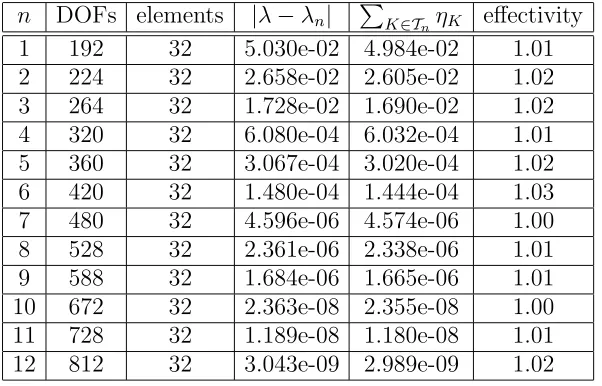
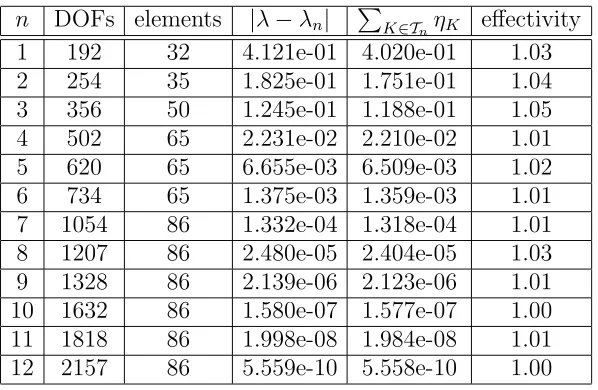
In Table 1 and Table 2 we have used Algorithm 1 to compute the first and the second eigenvalues. We note that the second eigenvalue 5π2 _{is degenerate—its corresponding}

in-variant subspace has dimension 2. The column DOFs contains the number of degrees of freedom in the finite element space Sn and the column elements contains the number of

elements in the mesh Tn. The last column contains the effectivity index which is defined as

|λ−λn|/|P_K∈TnηK|, which we see is very close to 1 even for our coarsest problems. In

Fig-ure 1 we plot |λ−λn| versus DOFs, and, as can be seen, the two graphs suggest exponential

convergence rate. The exceptional effectivity of the error estimator, and its apparent utility in guiding adaptive refinement, have been seen in other contexts as well (for example, fluid-dynamic problems in [22]), suggesting that functional error estimation and goal-oriented of this sort can have broad applicability.

n DOFs elements |λ−λn| P_K∈TnηK effectivity

[image:12.595.157.458.493.686.2]

1 192 32 5.030e-02 4.984e-02 1.01 2 224 32 2.658e-02 2.605e-02 1.02 3 264 32 1.728e-02 1.690e-02 1.02 4 320 32 6.080e-04 6.032e-04 1.01 5 360 32 3.067e-04 3.020e-04 1.02 6 420 32 1.480e-04 1.444e-04 1.03 7 480 32 4.596e-06 4.574e-06 1.00 8 528 32 2.361e-06 2.338e-06 1.01 9 588 32 1.684e-06 1.665e-06 1.01 10 672 32 2.363e-08 2.355e-08 1.00 11 728 32 1.189e-08 1.180e-08 1.01 12 812 32 3.043e-09 2.989e-09 1.02

Table 1. Results for the hp-adaptive method on the first eigenvalueλ = 2π2_.

(13)

[image:13.595.158.457.69.264.2]

1 192 32 4.121e-01 4.020e-01 1.03 2 254 35 1.825e-01 1.751e-01 1.04 3 356 50 1.245e-01 1.188e-01 1.05 4 502 65 2.231e-02 2.210e-02 1.01 5 620 65 6.655e-03 6.509e-03 1.02 6 734 65 1.375e-03 1.359e-03 1.01 7 1054 86 1.332e-04 1.318e-04 1.01 8 1207 86 2.480e-05 2.404e-05 1.03 9 1328 86 2.139e-06 2.123e-06 1.01 10 1632 86 1.580e-07 1.577e-07 1.00 11 1818 86 1.998e-08 1.984e-08 1.01 12 2157 86 5.559e-10 5.558e-10 1.00

Table 2. Results for the hp-adaptive method on the eigenvalue λ= 5π2_.

10 15 20 25 30 35 40 45 50 10−10

10−9 10−8 10−7 10−6 10−5 10−4 10−3 10−2 10−1 100

DOFs1/2

|

λ

−

λn

|

first eigenvalue second eigenvalue

Figure 1. Convergence of the first two eigenvalues for the Dirichlet Lapla-cian on the unit square.

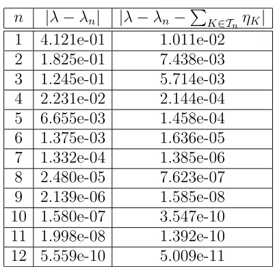
In situation such as that above, in which the effectivity of the estimator is near 1, Theo-rem 3.2 automatically suggests thatλn+PK∈TnηK is a better approximation ofλthan isλn.

This heuristic is validated in Tables 3-4, where we see decreases in error by one or two orders of magnitude! The principle of augmenting a computed eigenvalue with a highly-accurate error estimate is seen in other methods as well. In [35], the authors use gradient recovery techniques to improve their eigenvalue computations, and in [6] hierarchical basis techniques are used for the same purpose; in both cases, the approximation spaces Sn were conintuous

Lagrange elements of degree 1. Such “acceleration” procedures belong to a larger class of post-processing techniques, such as those used in [37, 42], in which the use of a finer space (in h or p) is common.

[image:13.595.177.425.318.512.2]

(14)

n |λ−λn| |λ−λn−P_K∈TnηK|

[image:14.595.207.406.69.265.2]

1 5.030e-02 4.568e-04 2 2.658e-02 5.289e-04 3 1.728e-02 3.880e-04 4 6.080e-04 4.815e-06 5 3.067e-04 4.668e-06 6 1.480e-04 3.620e-06 7 4.596e-06 2.202e-08 8 2.361e-06 2.289e-08 9 1.684e-06 1.837e-08 10 2.363e-08 8.970e-11 11 1.189e-08 8.851e-11 12 3.043e-09 5.453e-11

Table 3. Improved accuracy for the eigenvalueλ = 2π2_.

n |λ−λn| |λ−λn−PK∈TnηK|

1 4.121e-01 1.011e-02 2 1.825e-01 7.438e-03 3 1.245e-01 5.714e-03 4 2.231e-02 2.144e-04 5 6.655e-03 1.458e-04 6 1.375e-03 1.636e-05 7 1.332e-04 1.385e-06 8 2.480e-05 7.623e-07 9 2.139e-06 1.585e-08 10 1.580e-07 3.547e-10 11 1.998e-08 1.392e-10 12 5.559e-10 5.009e-11

Table 4. Improved accuracy for the eigenvalueλ = 5π2_.

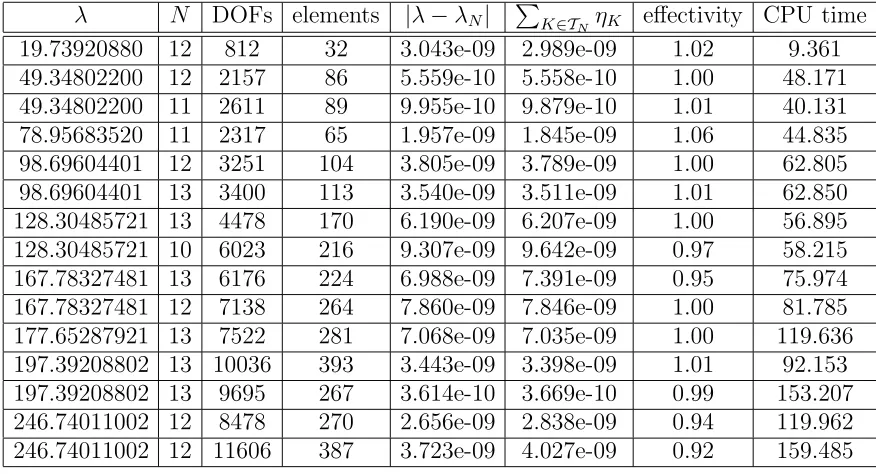
Finally, to more fully demonstrate the performance of Algorithm 1, in Table 5 we report, for the first 15 eigenvalues of the Laplace problem: the number of iterations N and degrees of freedom used to reach a precision of at least 1e−8, errors and effectivities on the finest mesh, and the total CPU time for the computation (in seconds).

[image:14.595.205.406.382.577.2]

(15)

λ N DOFs elements |λ−λN| P_K∈TNηK effectivity CPU time

[image:15.595.88.528.68.309.2]

19.73920880 12 812 32 3.043e-09 2.989e-09 1.02 9.361 49.34802200 12 2157 86 5.559e-10 5.558e-10 1.00 48.171 49.34802200 11 2611 89 9.955e-10 9.879e-10 1.01 40.131 78.95683520 11 2317 65 1.957e-09 1.845e-09 1.06 44.835 98.69604401 12 3251 104 3.805e-09 3.789e-09 1.00 62.805 98.69604401 13 3400 113 3.540e-09 3.511e-09 1.01 62.850 128.30485721 13 4478 170 6.190e-09 6.207e-09 1.00 56.895 128.30485721 10 6023 216 9.307e-09 9.642e-09 0.97 58.215 167.78327481 13 6176 224 6.988e-09 7.391e-09 0.95 75.974 167.78327481 12 7138 264 7.860e-09 7.846e-09 1.00 81.785 177.65287921 13 7522 281 7.068e-09 7.035e-09 1.00 119.636 197.39208802 13 10036 393 3.443e-09 3.398e-09 1.01 92.153 197.39208802 13 9695 267 3.614e-10 3.669e-10 0.99 153.207 246.74011002 12 8478 270 2.656e-09 2.838e-09 0.94 119.962 246.74011002 12 11606 387 3.723e-09 4.027e-09 0.92 159.485

Table 5. Results for the hp-adaptive on the first 15 eigenvalues for the Laplace problem on the unit square.

5.2. The L-Shaped Domain. A standard simple example for which (some of) the eigen-values and eigenfunctions are not explicitly known, and the eigenfunctions have reduced regularity, u /∈H2_{, is provided by the L-shaped domain}

Ω = [0,1]2\([0.5,1]×[0,0.5]),

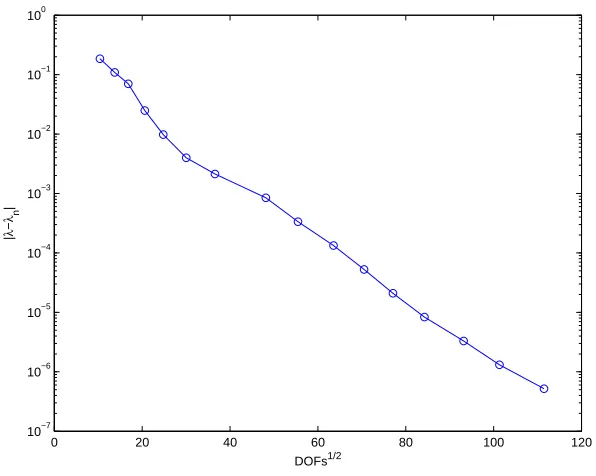
for which we again consider (5.1). The re-entrant corner at (0.5,0.5) causes some of the eigenfunctions to be singular there. This is certainly the case for the eigenfunctions associated with the smallest eigenvalue. The theory given in Section 3 does not cover such cases.

In Table 6 we have used Algorithm 1 to compute the first eigenvalue. The main difference between Table 6 and Table 1 (our analogous results for the unit square) is the fact that the effectivity index is in this case not close to 1, due to the singularity in the gradient of the first eigenfunction. Because of this, the auxiliary space ˜Sn constructed by DualSpace is not

“fine” enough for computing an approximation of z which is sufficient for estimating the error for eigenvalues to such a high level of accuracy. In this case the exact value of the eigenvalue is unknown, so in order to be able to compute the effectivity index, we use as a reference value, the eigenvalue computed at a very fine level. Despite this loss in effectivity, we see in Figure 2 that the convergence rate is still exponential. In Figure 3 we depict the final mesh with different colors to indicate different orders of polynomials. Unsurprisingly the elements are very small around the reentering corner, where the singularity sits and the orders of polynomials increase moving away from the singularity. The primary reason for including this example is to demonstrate that Algorithm 2 may be necessary in order to obtain effectivities near 1, and that this goal can in fact be achieved by using this variant. In Table 7 we have used Algorithm 2 withm= 2 to compute the first eigenvalue of the problem on the L-shaped domain. As can be seen the effectivity index is very close to 1 again, as in case of smooth problems. Comparing Table 7 with Table 6 it is clear that the difference

[image:15.595.86.524.71.308.2]

(16)

in the construction of the dual space has almost no effect on the convergence rate of the method, but just on the effectivity index. In Table 8 we compare the true error|λ−λn|with

the error for the improved estimation for the eigenvalueλn+P_K∈TnηK, based on Algorithm

2, where we again see an increase by one or two orders of magnitude.

n DOFs elements |λ−λn| PK∈TnηK effectivity

[image:16.595.158.455.420.672.2]

1 108 12 1.748e-01 1.847e-01 0.95 2 189 21 1.019e-01 1.087e-01 0.94 3 284 30 7.600e-02 7.003e-02 1.09 4 425 39 3.096e-02 2.480e-02 1.25 5 616 45 1.464e-02 9.804e-03 1.49 6 902 45 7.641e-03 3.995e-03 1.91 7 1339 45 4.903e-03 2.131e-03 2.30 8 2320 54 1.945e-03 8.446e-04 2.30 9 3078 63 7.718e-04 3.352e-04 2.30 10 4039 72 3.063e-04 1.330e-04 2.30 11 4971 81 1.215e-04 5.280e-05 2.30 12 5941 90 4.823e-05 2.095e-05 2.30 13 7100 99 1.914e-05 8.315e-06 2.30 14 8684 108 7.596e-06 3.300e-06 2.30 15 10268 117 3.014e-06 1.310e-06 2.30 16 12425 126 1.195e-06 5.198e-07 2.30

Table 6. Results for the hp-adaptive method on the first eigenvalue of the L-shape domain.

(17)

0 20 40 60 80 100 120 10−7

10−6 10−5 10−4 10−3 10−2 10−1 100

DOFs1/2

|

λ

−

λn

[image:17.595.153.451.86.324.2]

|

Figure 2. Convergence for first eigenvalue of the L-shape domain.

Figure 3. hp-adapted mesh for the L-shape domain.

[image:17.595.152.439.400.655.2]

(18)

[image:18.595.158.457.69.321.2]

1 108 12 1.748e-01 2.072e-01 0.84 2 189 21 1.019e-01 1.158e-01 0.88 3 284 30 7.600e-02 8.084e-02 0.94 4 425 39 3.096e-02 2.983e-02 1.04 5 616 45 1.464e-02 1.276e-02 1.15 6 902 45 7.641e-03 7.455e-03 1.02 7 1339 45 4.903e-03 4.642e-03 1.06 8 2045 54 1.945e-03 1.841e-03 1.06 9 2688 63 7.718e-04 7.306e-04 1.06 10 3437 72 3.063e-04 2.899e-04 1.06 11 4411 81 1.215e-04 1.151e-04 1.06 12 5434 90 4.823e-05 4.566e-05 1.06 13 6575 99 1.914e-05 1.812e-05 1.06 14 7862 108 7.596e-06 7.192e-06 1.06 15 9670 117 3.014e-06 2.854e-06 1.06 16 11548 126 1.195e-06 1.133e-06 1.06

Table 7. Results for the hp-adaptive method on the first eigenvalue of the L-shape domain using Algorithm 2.

n |λ−λn| |λ−λn−PK∈TnηK|

1 1.748e-01 3.240e-02 2 1.019e-01 1.386e-02 3 7.600e-02 4.845e-03 4 3.096e-02 1.135e-03 5 1.464e-02 1.876e-03 6 7.641e-03 1.856e-04 7 4.903e-03 2.612e-04 8 1.945e-03 1.037e-04 9 7.718e-04 4.116e-05 10 3.063e-04 1.633e-05 11 1.215e-04 6.481e-06 12 4.823e-05 2.571e-06 13 1.914e-05 1.020e-06 14 7.596e-06 4.041e-07 15 3.014e-06 1.597e-07 16 1.195e-06 6.278e-08

Table 8. Improved accuracy for the first eigenvalue of the L-shaped domain.

[image:18.595.206.406.432.686.2]

(19)

00000

11111

C

[image:19.595.248.365.72.192.2]

O

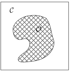
Figure 4. A generic composite two phased material.

5.3. Problems with a large coupling limit. As a first class of benchmark problems we consider the perturbation of the free Hamiltonian by a singular step potential, cf. Figure 4. The eigenvalue problem can be formulated as

AOκψ :=−△ψ+κχO ·ψ =λψ, (5.2)

ψ ∈H01(Ω),kψk0 = 1.

(5.3)

Here Ω⊂ R2 _{is bounded, connected and open, and} _χO _{is the characteristic function of the}

set O ⊂Ω. Alternatively we can set C = Ω\ O and study the problem ACκψ :=−△ψ+κχC ·ψ =λψ,

(5.4)

ψ ∈H₀1(Ω),kψk0 = 1.

(5.5)

The second problem models a waveguide type problem, whereas the first is characteristic of the hard-core scattering problems. Furthermore, such short range potentials appear fre-quently in the study of the spectral properties of disordered media [8, 10, 17, 41]. Similarly formulated problems appear also in the study of optical wave-guides and other nano-devices (see [11, 33]). For any given κ > 0, the eigenvalue problems (5.2) and (5.4) are of the sort considered in [21], where convergence of several adaptive methods for eigenvalue problems was proved. A third type of problem, for which the jump discontinuity is in the derivative, will also be discussed below. Analyzing and understanding the spectra of such problems is a key ingredient in the inverse spectral theory behind nondestructive sensing methods described in [1, 2].

Remark 5.1. If Ω is convex and O ⊂ Ω is measurable, then all eigenfunctions ψ associated with eigenvalue problems of the form

−∆ψ +κχO ·ψ =λψ , ψ∈H₀1(Ω) , kψk0 = 1

are in H2

A=H2(Ω). In particular, this holds for problems (5.2) and (5.4) in this subsection, as well as for problems (5.10) and (5.12) in Subsection 5.4. This fact is apparent from well-known regularity theory for boundary value problems when one notes that −∆ψ = (λ−κχO)ψ ∈L2_(Ω).

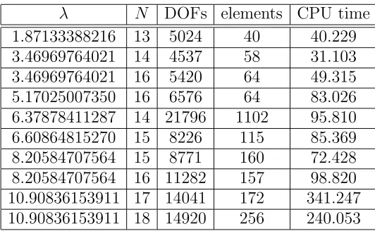
For the simulations described in Tables 9-10, we set Ω = [−2,2]2_, _O _{= [}₋_1,_1]2 _and _κ_{= 1.}

In both cases, Algorithm 1 is used, and since the true eigenvalues are not known, we stop when the error estimator

P

K∈TnηK

(20)

[image:20.595.172.438.69.233.2]

λ N DOFs elements CPU time 1.87133388216 13 5024 40 40.229 3.46969764021 14 4537 58 31.103 3.46969764021 16 5420 64 49.315 5.17025007350 16 6576 64 83.026 6.37878411287 14 21796 1102 95.810 6.60864815270 15 8226 115 85.369 8.20584707564 15 8771 160 72.428 8.20584707564 16 11282 157 98.820 10.90836153911 17 14041 172 341.247 10.90836153911 18 14920 256 240.053

Table 9. Results for thehp-adaptive on the first 10 eigenvalues of (5.2) with κ= 1.

[image:20.595.171.439.287.450.2]

Table 10. Results for the hp-adaptive on the first 10 eigenvalues of (5.4) with κ= 1.

A second type of problem considered here has its jump discontinuity on the second-derivative term, and is given formally by,

Tκψ :=−∇ ·[(1 +κχC)∇] ψ =λψ, (5.6)

ψ ∈H₀1(Ω),kψkH0 = 1.

(5.7)

As a test example, we consider Ω = (−1,1)2 _with _C _{= (}₋_1,₁₎_×_(0,_{1). The structure of}

the domain and differential operator is such that the eigenvalues and eigenfunctions may be computed by (partially) analytic means. In particular, using separation-of-variables and continuity of both the eigenfunction and its flux across the interface between C and its complement, we deduce that all eigenfunctions are inH_{A(Ω), and the eigenvalues are of one}2

of two types:

I) For m∈N _and _λ _∈₍π2m

4 , (1 +κ) π2

m

4 ), we define

Km =

r

λ− π2m

4 , Lm =

r

π2_m

4 − λ 1 +κ .

(21)

Any admissable λ which satisfies

(1 +κ)LncoshLn sinKn+KncosKn sinhLn= 0

is an eigenvalue ofTκ.

II) For m∈N _and _{λ >}_{(1 +}_κ)π2m

4 , we define Km as before, and

Mm =

r

λ 1 +κ −

π2_m

4 . Any admissable λ which satisfies

(1 +κ)MncosMn sinKn+KncosKn sinMn= 0

is an eigenvalue of Tκ.

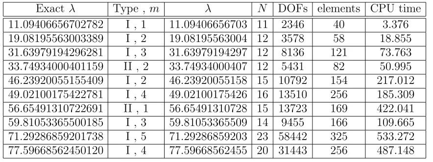
Choosing and m and κ, these equations can be solved with extremely high accuracy and precision using a computer algebra system. In Table 11 we provide data for the first 10 eigenvalues of (5.6) for κ = 9, using Algorithm 1 and stopping when the error estimator

P

K∈TnηK

goes below 1e−10. We include the exact eigenvalues to full 16-digit accuracy

(rounded) together with our computed approximations at termination of the algorithm. As is apparent, each of the computed eigenvalues is accurate to (at least) 10 digits.

[image:21.595.87.529.361.527.2]

Exact λ Type , m λ N DOFs elements CPU time 11.09406656702782 I , 1 11.09406656703 11 2346 40 3.376 19.08195563003389 I , 2 19.08195563004 12 3578 58 18.855 31.63979194296281 I , 3 31.63979194297 12 8136 121 73.763 33.74934000401159 II , 2 33.74934000407 12 5431 82 50.995 46.23920055155409 I , 2 46.23920055158 15 10792 154 217.012 49.02100175422781 I , 4 49.02100175426 16 13510 256 185.309 56.65491310722691 II , 1 56.65491310728 15 13723 169 422.041 59.81053365500185 I , 3 59.81053365509 14 9455 166 109.665 71.29286859201738 I , 5 71.29286859203 23 58442 325 533.272 77.59668562450120 I , 4 77.59668562455 20 31443 256 487.148

5.3.1. A computational study of the large coupling limit. We finally turn to examples which give this subsection its name—those for which we investigate the asymptotic behavior of the spectra of the operators AC

κ and T

C

κ as κ → ∞. To this end let λκ1 ≤ λκ2 ≤ · · · and

µκ

1 ≤µκ2 ≤ · · · be the ordered eigenvalues of the operators A

C

κ and T

C

κ, respectively, counted

according to multiplicity. Furthermore, let λ∞

1 ≤ λ

∞

2 ≤ · · · denote the eigenvalues of the

limit operator A∞, which is, in both cases, defined by A∞ψ =−∆ψ =λψ, (5.8)

ψ ∈H₀1(O),kψkH1

0 = 1.

(5.9)

(22)

According to the theory from [8, 11, 17, 23, 38] λκ i → λ

∞

i and µκi → λ

∞

i as κ → ∞. The

difference is in the convergence rates. According to [23] we have

|µκ i −λ

∞

i |

λ∞

i

=O(κ−1), i∈N

for any problem of the type (5.6), but for problems of the type (5.4) we have

|λκ i −λ

∞

i |

λ∞

i

=O(κ−α), i∈N

for some α ∈(0,1]. The parameter α depends on the regularity properties of the boundary ∂O. This analysis is much more involved (cf. [26]), and we consider it empirically in Table 12 for the first eigenvalue of (5.4). In Table 12-(a) we estimate the value of α for the first eigenvalue of problem (5.6) for a sequence of values of κ, recalling that, for problem (5.6),λ∞

1 =π2+ (π/2)2. In Table 12-(b) we estimate the value ofαfor the first eigenvalue of

problem (5.4) for a sequence of values of κ, we recalling that, for problem (5.4),λ∞

1 = 2π2.

κ α

1.0e+01 -1.0e+02 0.950 1.0e+03 0.996 1.0e+04 1.000 1.0e+05 1.000 1.0e+06 1.000 1.0e+07 1.000 1.0e+08 1.000

κ α

1.0e+01 -1.0e+02 0.276 1.0e+03 0.447 1.0e+04 0.486 1.0e+05 0.496 1.0e+06 0.499 1.0e+07 0.500 1.0e+08 0.500

[image:22.595.213.400.295.441.2]

(a) (b)

Table 12. Estimations for the exponent α for problem (5.6) and for the problem for problem (5.4).

5.4. Benchmarking the adaptivity of eigenvalue methods. Two key constants related to the quality of a posteriori error estimates for eigenvalue problems are

(1) The stability constant Cstb, measuring the distance to the unwanted component of

the spectrum.

(2) The regularity constant Creg, measuring the regularity properties of the

eigenfunc-tions.

In our basic estimator result from Corollary 3.3 the stability constants are implicit in the assumption that the dual problem is well-posed and the assumption that we need H2

A reg-ularity to establish rigorous convergence results. In this section we present two parameter dependent examples where either H2

A regularity is violated or the eigenvalue clustering is increased as a controlled function of the problem parameter. This gives us an opportunity to both generate an interesting benchmark—e.g. one which is close to violating either the requirement (1) or (2) in a controlled way—and to use the analytical knowledge of the spec-tral behavior of the eigenvalues in the parameter limit in order to circumstantially validate the method.

(23)

For a discussion of the roll played by these constants in eigenvalue estimates see [34, 5]. The reference [5] is particularly interesting as a motivation for providing accurate benchmark eigenvalues for use in experimental studies and for gaining insight in situations where one does not have an analytical option. We have illustrated a potential of our method in this experimental context in Section 5.3.1 and will do so again for the following two problems.

5.4.1. Problems with an asymptotic doubling of the multiplicity. As a prototype example in this class we consider the family of problems

− △ψ+κVM D·ψ =λψ,

(5.10)

ψ ∈H₀1([−1,1]2),kψk0 = 1.

(5.11)

where the function VM D is defined as the characteristic function of the coalescent squares

which are denoted by M1 in Figure 5. This example was originally proposed and solved as

a test example for an eigenvalue problem un electromagnetism by M. Dauge in [16]. In its original formulation the problem is much more challenging, since the jumps are contained in the second order therm, cf. [16]. A similar problem — having jumps in the second order term — has also been studied as an interesting example in the context of ill-posed boundary value problems by Knyazev and Widlund in [32]. There, an extensive regularity theory for such problems is presented as well.

In Table 13 we provide data for the first 10 eigenvalues of (5.10) with κ = 1 using Al-gorithm 1. Again, the exact eigenvalues for this problem eigenvalues are not known, so we stop when the

P

K∈TnηK

goes below 1e−10.

[image:23.595.172.439.510.674.2]

(24)

000000

111111

000000

111111

M2

M1

[image:24.595.220.392.71.245.2]

M1

Figure 5. A modification of the touching squares example of M. Dauge. The potential VM D is the characteristic function of the coalescent squares denoted

by VM D.

According to the theory from [8, 11, 17, 23, 38], as κ → ∞ we have that the smallest two eigenvalues of (5.10), λκ

1 and λκ2, with are distinct for any finite κ, both converge to

the double eigenvalue 2π2 _{of the Dirichlet Laplace eigenvalue problem posed in the domain}

consisting of the two unit squares labelled M2 in Figure 5. Additionally, it holds that

|λκ

1 −2π2|

2π2 =O κ

−_α

, |λ

κ

2 −2π2|

2π2 =O κ

−_α

.

We will estimate 0< α≤1 by fitting the computed error estimates. Furthermore, this will serve as an indirect check of our accuracy claims. The theory from [11] does not cover this case, but we formally expect that α = 1/2. In Table 14-(a)and Table 14-(b) we give our estimated values of αfor the first two eigenvalues of problem (5.10) for a sequence of values of κ.

κ α

1.0e+01 -1.0e+02 0.469 1.0e+03 0.486 1.0e+04 0.488 1.0e+05 0.496 1.0e+06 0.499 1.0e+07 0.500

κ α

1.0e+01 -1.0e+02 0.276 1.0e+03 0.447 1.0e+04 0.486 1.0e+05 0.496 1.0e+06 0.499 1.0e+07 0.500 1.0e+08 0.500

(a) (b)

Table 14. Estimations for the exponent α for the first eigenvalue of (5.10) and for the second eigenvalue.

[image:24.595.213.400.523.671.2]

(25)

00 00 00 11 11 11

00 00 00 00

[image:25.595.210.403.71.158.2]

11 11 11 11

Figure 6. A dumbbell example. The region C is shaded. 5.4.2. Problems with an asymptotic loss of H2

A regularity. We consider the problem

− △ψ+κχC·ψ =λψ, (5.12)

ψ ∈H01(Ω),kψk0 = 1.

(5.13)

where Ω is the rectangular domain pictured in Figure 6, and C is the shaded region. In the limit as κ → ∞ we obtain the dumbbell example from [9], where the domain consists of two π×π squares coupled by a π

4 × π

4 square “bridge”. In Table 15 we provide data for the

first 10 eigenvalues of (5.12) with κ= 1, using Algorithm 1. Moreover, in Table 16 we show the convergence of the first 10 eigenvalues of (5.12) to the limit problem as κ → ∞. The quantities βi are defined as

βi :=

|λi−λ∞i |

λ∞

i

,

where λi = λκi are the eigenvalues of (5.12) and λ

∞

i are the corresponding eigenvalues of

the Dirichlet Laplacian on the dumbbell domain, ordered accoring to multiplicity. Also, in Table 17 we give estimates of the rate of convergence of the first 10 eigenvalues, where

βi =O(κ

−αi

).

We note that the eigenfunction(s) of (5.12) associated with λi =λκi are in HA2 for all i and all (finite) κ; but the eigenfunction(s) of the Dirichlet Laplacian on the dumbbell domain associated with λ∞

i are generally not in HA.2

[image:25.595.173.440.511.674.2]

(26)

κ β1 β2 β3 β4 β5 β6 β7 β8 β9 β10

[image:26.595.99.515.255.376.2]

1.0e+00 0.687 0.350 0.572 0.359 0.230 0.353 0.271 0.414 0.287 0.281 1.0e+01 0.521 0.293 0.368 0.287 0.206 0.160 0.234 0.301 0.242 0.175 1.0e+02 0.240 0.153 0.132 0.129 0.124 0.072 0.073 0.081 0.093 0.073 1.0e+03 0.087 0.058 0.045 0.045 0.050 0.028 0.025 0.029 0.029 0.026 1.0e+04 0.029 0.020 0.015 0.015 0.017 0.009 0.008 0.010 0.009 0.009 1.0e+05 0.009 0.006 0.005 0.005 0.006 0.003 0.003 0.003 0.003 0.003 1.0e+06 0.003 0.002 0.002 0.002 0.002 0.001 0.001 0.001 0.001 0.001

Table 16. Convergence of the first 10 eigenvalues of (5.12) to those of the dumbbell problem as κ increases.

κ α1 α2 α3 α4 α5 α6 α7 α8 α9 α10

1.0e+00 - - -

-1.0e+01 0.121 0.077 0.192 0.098 0.048 0.345 0.065 0.139 0.075 0.207 1.0e+02 0.336 0.283 0.445 0.346 0.221 0.343 0.507 0.568 0.417 0.381 1.0e+03 0.440 0.422 0.463 0.457 0.396 0.417 0.459 0.453 0.508 0.446 1.0e+04 0.477 0.470 0.485 0.484 0.465 0.472 0.480 0.477 0.492 0.481 1.0e+05 0.490 0.488 0.494 0.494 0.489 0.491 0.493 0.491 0.495 0.492 1.0e+06 0.495 0.494 0.497 0.497 0.496 0.497 0.498 0.496 0.497 0.496

Table 17. Rate of convergence of the first 10 eigenvalues of (5.12) to those of the dumbbell problem as κ increases.

Acknowledgement

L. G. was supported by the grant: “Spectral decompositions – numerical methods and applications”, Grant Nr. 037-0372783-2750 of the Croatian MZOS.

We would like to thanks Paul Houston and Edward Hall for kind support and very useful discussions.

References

[1] H. Ammari, Y. Capdeboscq, H. Kang, and A. Kozhemyak. Mathematical models and reconstruction methods in magneto-acoustic imaging.European J. Appl. Math., 20(3):303–317, 2009.

[2] H. Ammari, H. Kang, E. Kim, and H. Lee. Vibration testing for anomaly detection. Math. Methods Appl. Sci., 32(7):863–874, 2009.

[3] H. Ammari, H. Kang, and H. Lee. Asymptotic analysis of high-contrast phononic crystals and a criterion for the band-gap opening.Arch. Ration. Mech. Anal., 193(3):679–714, 2009.

[4] D. Arnold, F. Brezzi, B. Cockburn, and L. Marini. Unified analysis of discontinuous galerkin methods for elliptic problems.SIAM J. Numer. Anal., 24(3):1749–1779, 2001.

[5] L. Banjai, S. B¨orm, and S. Sauter. FEM for elliptic eigenvalue problems: how coarse can the coarsest mesh be chosen? An experimental study.Comput. Vis. Sci., 11(4-6):363–372, 2008.

[6] R. Bank, L. Grubiˇsi´c, and J. S. Ovall. A framework for robust eigenvalue and eigenvector error estimation and ritz value convergence enhancement.MPI-MSI Preprint 42, 2010.

[7] R. Becker and R. Rannacher. An optimal control approach to a posteriori error estimation in finite element methods.Acta Numer., 10:1–102, 2001.

(27)

[8] A. Ben Amor and J. F. Brasche. Sharp estimates for large coupling convergence with applications to Dirichlet operators.J. Funct. Anal., 254(2):454–475, 2008.

[9] T. Betcke and L. N. Trefethen. Reviving the method of particular solutions.SIAM Rev., 47(3):469–491 (electronic), 2005.

[10] J. F. Brasche, R. Figari, and A. Teta. Singular Schr¨odinger operators as limits of point interaction Hamiltonians.Potential Anal., 8(2):163–178, 1998.

[11] V. Bruneau and G. Carbou. Spectral asymptotic in the large coupling limit.Asymptot. Anal., 29(2):91– 113, 2002.

[12] L.-Q. Cao and J.-Z. Cui. Asymptotic expansions and numerical algorithms of eigenvalues and eigenfunc-tions of the Dirichlet problem for second order elliptic equaeigenfunc-tions in perforated domains.Numer. Math., 96(3):525–581, 2004.

[13] L.-Q. Cao and J.-L. Luo. Multiscale numerical algorithm for the elliptic eigenvalue problem with the mixed boundary in perforated domains.Appl. Numer. Math., 58(9):1349–1374, 2008.

[14] A. Cliffe, E. Hall, P. Houston, E. T. Phipps, and A. G. Salinger. Adaptivity and a posteriori error control for bifurcation problems ii: Incompressible fluid flow in open systems withz₂symmetry.Journal of Scientific Computing, (submitted). URL: http://eprints.nottingham.ac.uk/1257/.

[15] K. A. Cliffe, E. J. Hall, and P. Houston. Adaptive discontinuous Galerkin methods for eigenvalue problems arising in incompressible fluid flows.SIAM J. Sci. Comput., 31(6):4607–4632, 2009/10. [16] M. Dauge. Benchmark collection, retrieved on March 31st 2010. URL:

http://perso.univ-rennes1.fr/monique.dauge/benchmax.html.

[17] M. Demuth, F. Jeske, and W. Kirsch. Quantitative estimates for Schrödinger and Dirichlet semigroups. InJournées “ Équations aux Dérivées Partielles” (Saint-Jean-de-Monts, 1992), pages Exp. No. XVII, 6. École Polytech., Palaiseau, 1992.

[18] M. Demuth and M. Krishna.Determining spectra in quantum theory, volume 44 ofProgress in Mathe-matical Physics. Birkh¨auser Boston Inc., Boston, MA, 2005.

[19] T. Eibner and J. Melenk. An adaptive strategy for hp-fem based on testing for analyticity.Comp. Mech., 39:575–595, 2007.

[20] A. Ern, A. F. Stephansen, and P. Zunino. A discontinuous Galerkin method with weighted averages for advection-diffusion equations with locally small and anisotropic diffusivity. IMA J. Numer. Anal., 29(2):235–256, 2009.

[21] E. M. Garau, P. Morin, and C. Zuppa. Convergence of adaptive finite element methods for eigenvalue problems.Math. Models Methods Appl. Sci., 19(5):721–747, 2009.

[22] S. Giani and P. Houston. ADIGMA - A European Initiative on the Development of Adaptive Higher-Order Variational Methods for Aerospace Applications, chapter 28, pages 399–411. Springer, 2010. [23] L. Grubiˇsi´c. Relative convergence estimates for the spectral asymptotic in the large coupling limit.

Integral Equations Operator Theory, 65(1):51–81, 2009.

[24] R. Hartmann and P. Houston. Adaptive discontinuous Galerkin finite element methods for nonlinear hyperbolic conservation laws.SIAM J. Sci. Comput., 24(3):979–1004, 2002.

[25] R. Hartmann and P. Houston. An optimal order interior penalty discontinuous Galerkin discretization of the compressible Navier–Stokes equations.J. Comp. Phys., 227:9670–9685, 2008.

[26] R. Hempel and O. Post. Spectral gaps for periodic elliptic operators with high contrast: an overview. In

Progress in analysis, Vol. I, II (Berlin, 2001), pages 577–587. World Sci. Publ., River Edge, NJ, 2003. [27] P. D. Hislop and O. Post. Anderson localization for radial tree-like quantum graphs. Waves Random

Complex Media, 19(2):216–261, 2009.

[28] P. Houston, D. Sch¨otzau, and T. Wihler. Energy norm a posteriori error estimation of hp–adaptive discontinuous Galerkin methods for elliptic problems.Math. Mod. Meth. Appl. Sci., 17(1):33–62, 2007. [29] P. Houston, C. Schwab, and E. S¨uli. Discontinuous hp-finite element methods for

advection-diffusion-reaction problems.SIAM J. Numer. Anal., 39(6):2133–2163, 2002.

[30] P. Houston and E. S¨uli. A note on the design of hp-adaptive finite element methods for elliptic partial differential equations.Comput. Methods Appl. Mech. Engrg., 194(2-5):229–243, 2005.

[31] T. Kato. Perturbation theory for linear operators. Classics in Mathematics. Springer-Verlag, Berlin, 1995. Reprint of the 1980 edition.

(28)

[32] A. Knyazev and O. Widlund. Lavrentiev regularization + Ritz approximation = uniform finite ele-ment error estimates for differential equations with rough coefficients. Math. Comp., 72(241):17–40 (electronic), 2003.

[33] T. Koprucki, R. Eymard, and J. Fuhrmann. Convergence of a finite volume scheme to the eigenvalues of a schroedinger operator. Technical report, WIAS Preprint No. 1260, 2007.

[34] M. G. Larson. A posteriori and a priori error analysis for finite element approximations of self-adjoint elliptic eigenvalue problems.SIAM J. Numer. Anal., 38(2):608–625 (electronic), 2000.

[35] A. Naga, Z. Zhang, and A. Zhou. Enhancing eigenvalue approximation by gradient recovery.SIAM J. Sci. Comput., 28(4):1289–1300 (electronic), 2006.

[36] I. Perugia and D. Sch¨otzau. The hp-local discontinuous Galerkin method for low-frequency time-harmonic Maxwell equations.Math. Comp., 72(243):1179–1214, 2003.

[37] M. R. Racheva and A. B. Andreev. Superconvergence postprocessing for eigenvalues.Comput. Methods Appl. Math., 2(2):171–185, 2002.

[38] E. S´anchez-Palencia. Asymptotic and spectral properties of a class of singular-stiff problems.J. Math. Pures Appl. (9), 71(5):379–406, 1992.

[39] S. Sauter. hp-finite elements for elliptic eigenvalue problems: error estimates which are explicit with respect toλ,h, andp.SIAM J. Numer. Anal., 48(1):95–108, 2010.

[40] D. Sch¨otzau and L. Zhu. A robust a-posteriori error estimator for discontinuous galerkin methods for convection-diffusion equations.Appl. Numer. Math., 59:2236–2255, 2009.

[41] P. Stollmann.Caught by disorder, volume 20 ofProgress in Mathematical Physics. Birkh¨auser Boston Inc., Boston, MA, 2001. Bound states in random media.

[42] J. Xu and A. Zhou. A two-grid discretization scheme for eigenvalue problems. Math. of Comput., 70(233):17–25, 2001.

[43] L. Zhu, S. Giani, P. Houston, and D. Sch¨otzau. Energy norm a-posteriori error estimation forhp-adaptive discontinuous galerkin methods for eliptic problems in three dimensions.Math. Models Methods Appl. Sci., (to appear), 2011.

School of Mathematical Sciences University of Nottingham , University Park, Notting-ham, NG7 2RD, United Kingdom

E-mail address: [email protected]

University of Zagreb, Department of Mathematics, Bijeniˇcka 30, 10000 Zagreb, Croatia

University of Kentucky, Department of Mathematics, Patterson Office Tower 761, Lex-ington, KY 40506-0027, USA